

EN
Introduction
This section focuses on the concept of sequence modeling and how to construct neural networks that can handle and learn from sequential data. The lecture begins by introducing the importance of sequence modeling in understanding and processing data involving sequence handling, such as language, audio, financial markets, and biological sequences.
The significance of understanding the foundational functions of neural networks and developing intuition in the context of sequence modeling is emphasized. The concept of recurrence is introduced, explaining how Recurrent Neural Networks (RNNs) are designed to process sequential data. This includes understanding the network’s internal state or memory and how it updates over time as new data is processed.
Object Trajectories

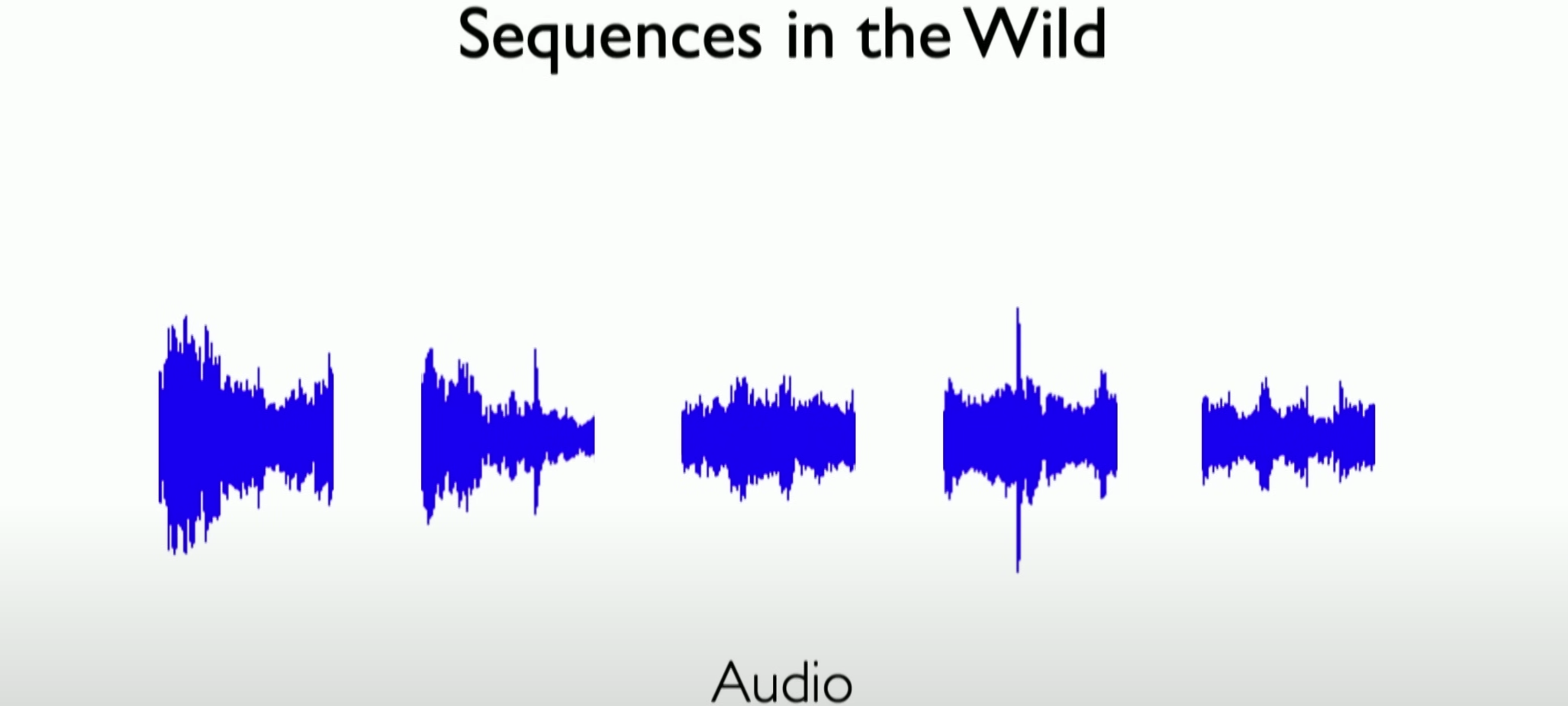
Sound Waves
Language
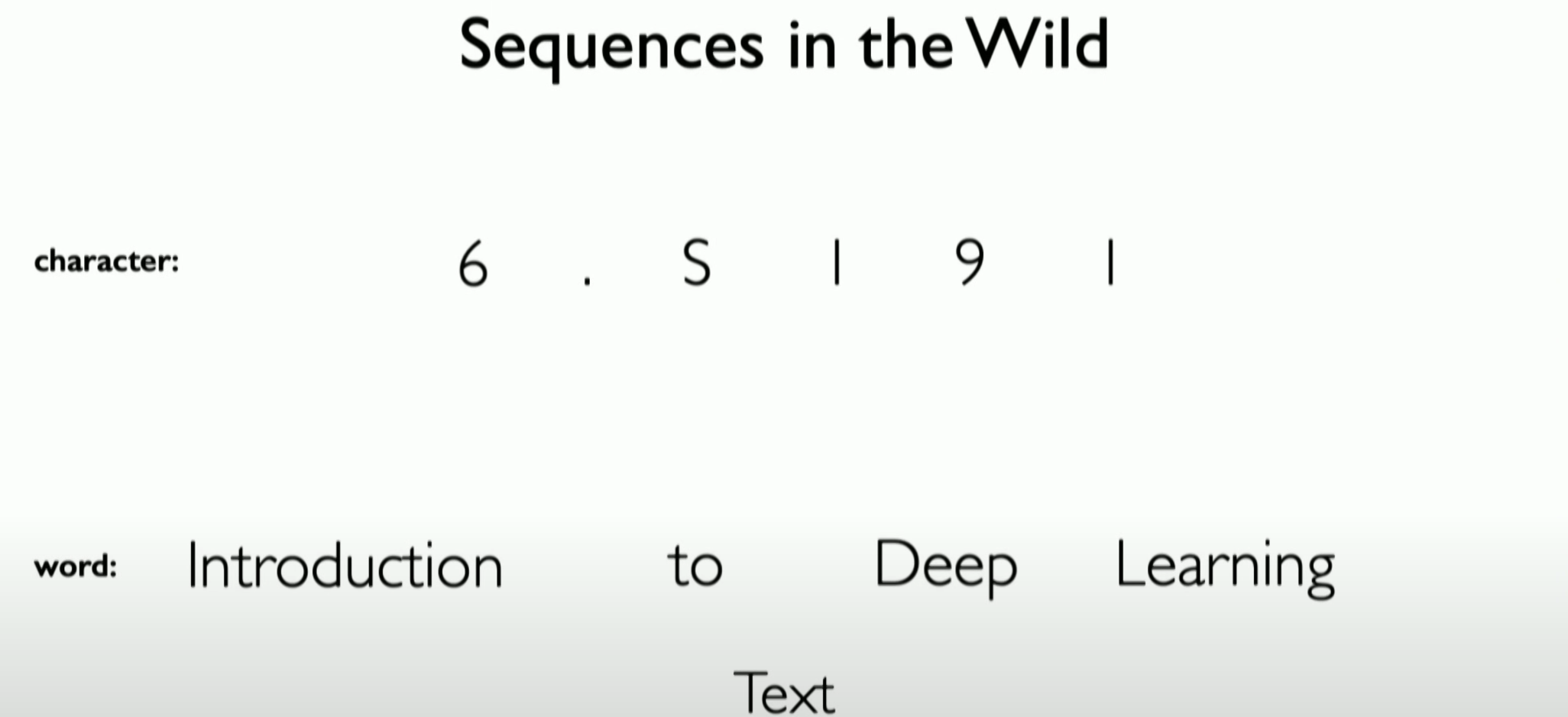
The presence of sequential data in everyday environments is illustrated through practical examples, such as the trajectory of moving objects, sound waves, and language. These examples highlight the relevance of sequence modeling in real-world applications. Next, the concept of embedding is explained, which is crucial for converting textual data into a numerical format that neural networks can process.
Key design criteria for RNNs, such as handling variable sequence lengths, tracking dependencies over time, and maintaining the order in sequences, are also covered. The discussion includes how these design criteria inspire the need for robust architectures like Transformers, which can outperform RNNs in sequence modeling tasks.
Finally, the training process of RNNs is discussed, focusing on the backpropagation algorithm and its adaptation to sequence data, known as backpropagation through time. This part highlights the technical details involved in effectively training RNNs for handling sequential data.
Sequence Modeling
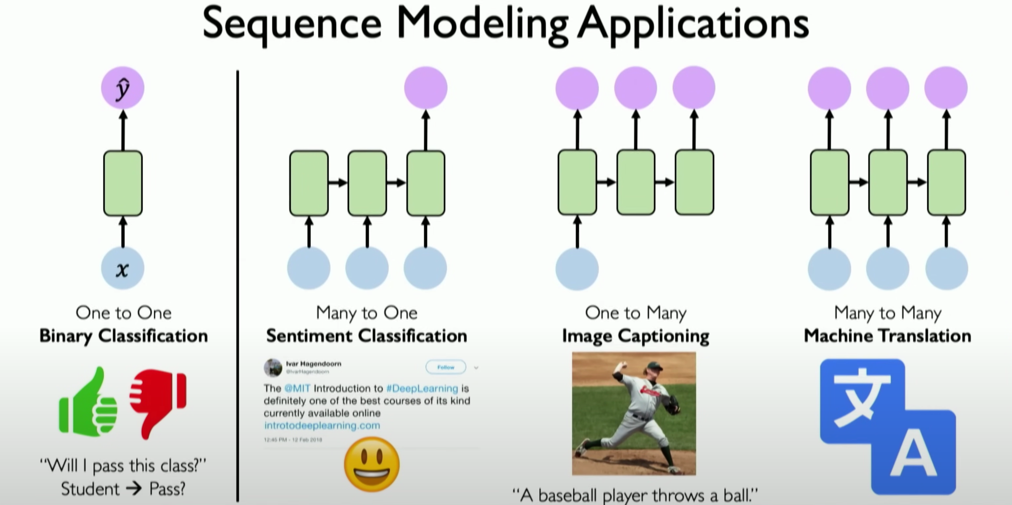
Sequence modeling has various applications. We can roughly classify them based on their input and output: one-to-one (binary classification problem), many-to-one, one-to-many, and many-to-many problems.
The second part focuses on sequence modeling, exploring the principles and applications of Recurrent Neural Networks (RNNs), Long Short-Term Memory networks (LSTMs), and attention mechanisms.
Importance of Sequence Modeling: Sequence modeling is crucial for understanding how neural networks handle sequences of varying lengths. This includes tracking dependencies in sequences of different lengths, such as maintaining the relevance of early information in long sentences.
Neurons with Recurrence
The “Neurons with Recurrence” section covers the following aspects:
The Concept of Recurrence and Definition of Recurrent Neural Networks: The concept of recurrence is introduced first to build an understanding of Recurrent Neural Networks (RNNs). RNNs are powerful tools for handling sequential data.
From Perceptron to Recurrent Neural Networks: The course starts with the basic concept of a perceptron and explains how to extend the idea of neural networks by adding recurrence. A perceptron is a single neuron operation where multiple inputs are multiplied by corresponding weights and generate output through a nonlinear activation function. In traditional perceptrons or feedforward neural networks, the time sequence or sequential nature of input data is not considered.
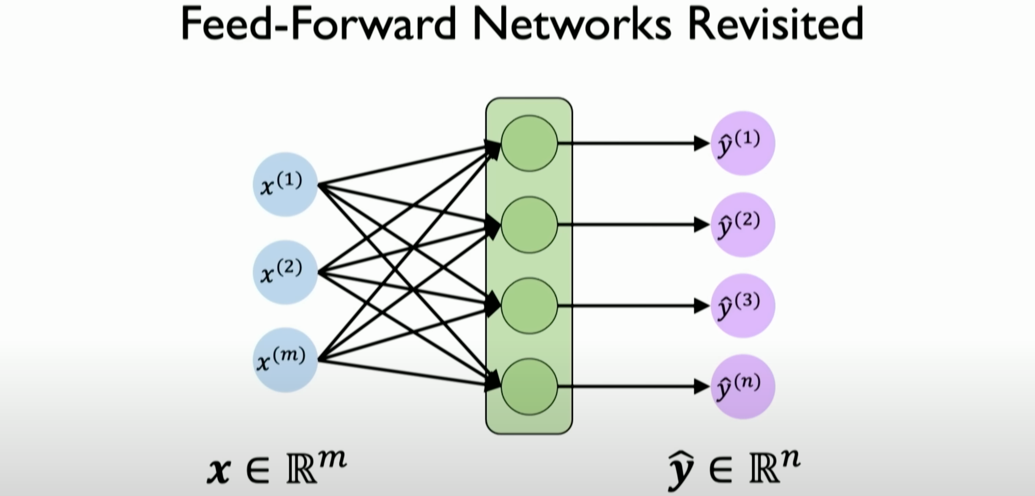
In the case of feedforward neural networks, even if multiple perceptrons are stacked together, there is still no concept of temporal processing or sequential information.
The Concept of Time Steps and Internal States: The concept of time steps is introduced, which is key to understanding RNNs. RNNs consider time steps when processing data, meaning the network’s output depends on current input data and the past internal state or memory.
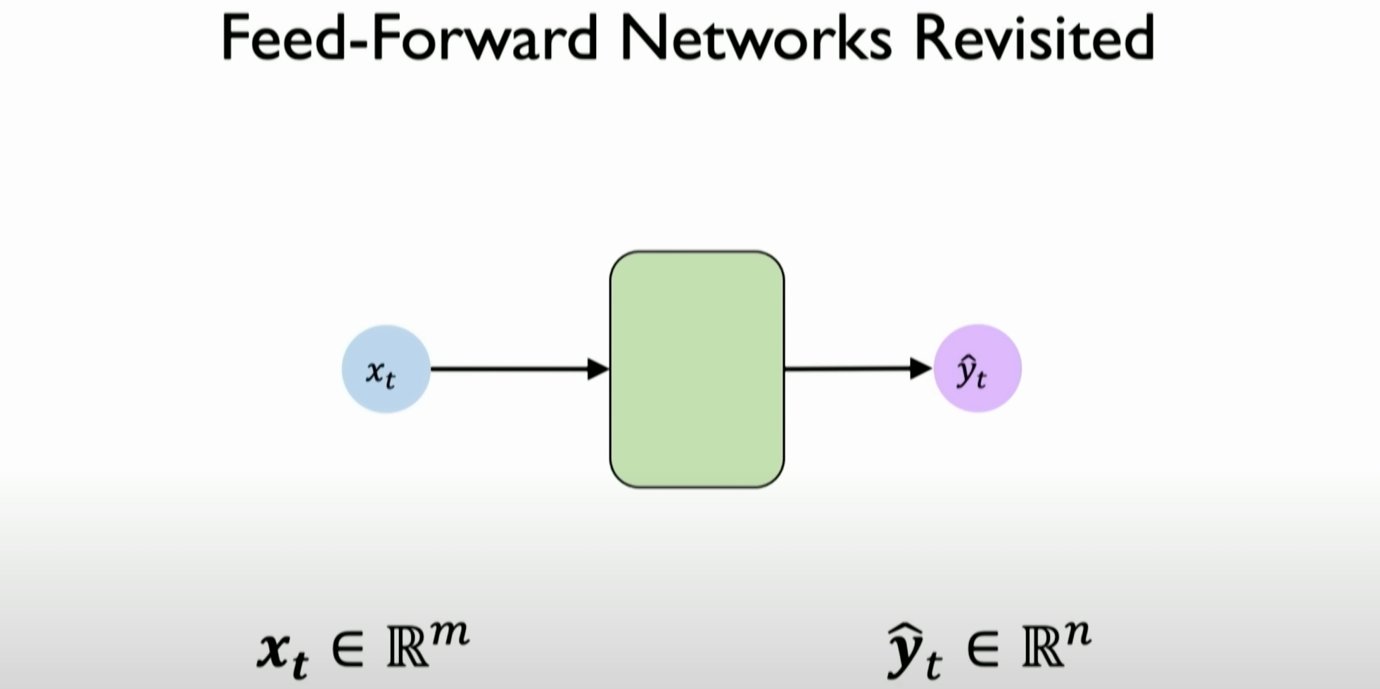
We attempt to simplify the process of inputs and outputs through perceptrons using a simple green block without changing any processing inside it. We introduce a new variable
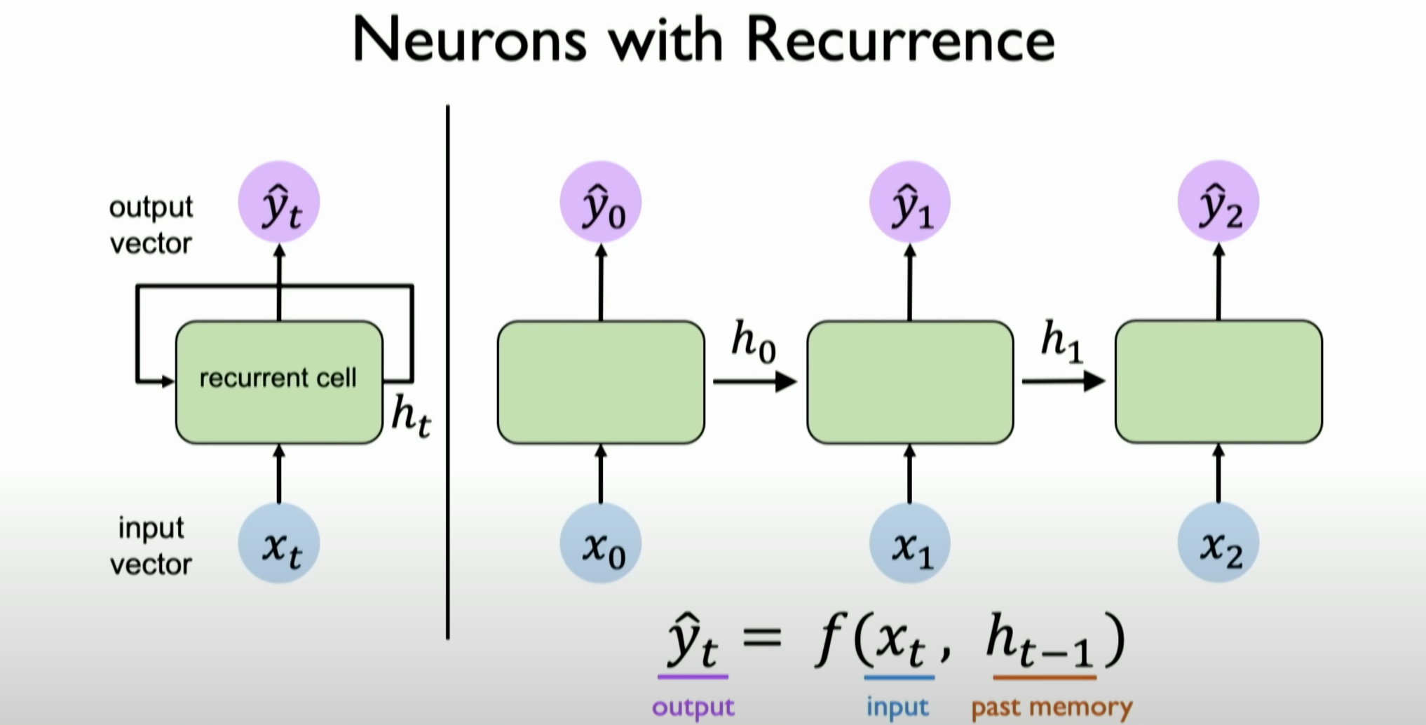
Tto represent a single time step.Recurrence Relations and Internal State Updates: RNNs maintain and update their internal state through recurrence relations. This recurrence relation determines how the network’s computation at a specific time step is carried forward to subsequent time steps. The internal state update is mathematically similar to other neural network operations but considers the current input and the previous time step’s state.
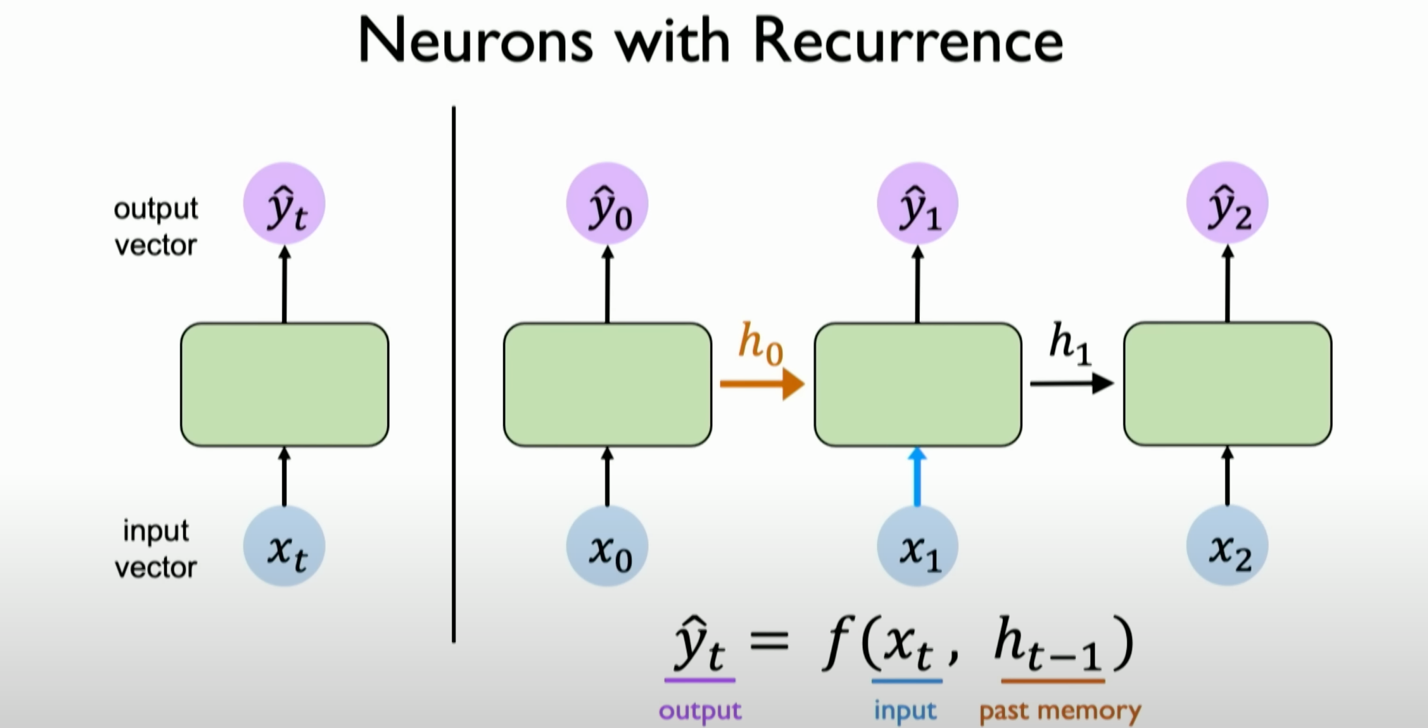
Here, we define a variable
H, known as the internal state, maintained by neurons and the network. It is inputted along with the sequence information, capturing the memory concept and dynamically changing as it passes through the neural network.Unfolding the Computation Graph of RNNs: The computation graph of RNNs is explained, showing how each time step is processed independently and accumulated to form the overall output.
Recurrent Neural Networks
Mathematical Definition and Implementation of RNNs: The mathematical definition of RNNs and how to implement them in code is described in detail. The emphasis is on how RNNs work by maintaining state and updating it with each sequence processing step.
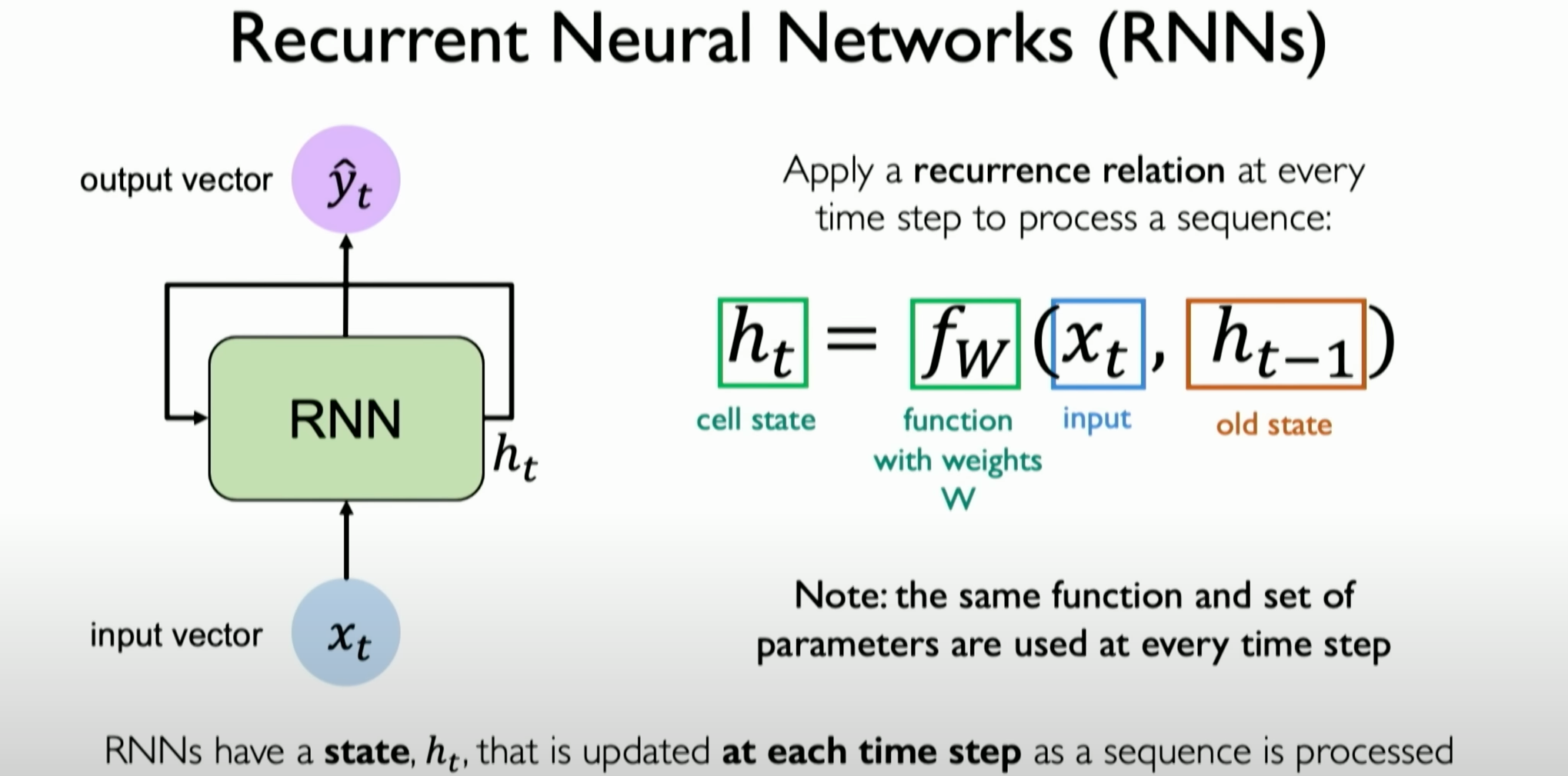
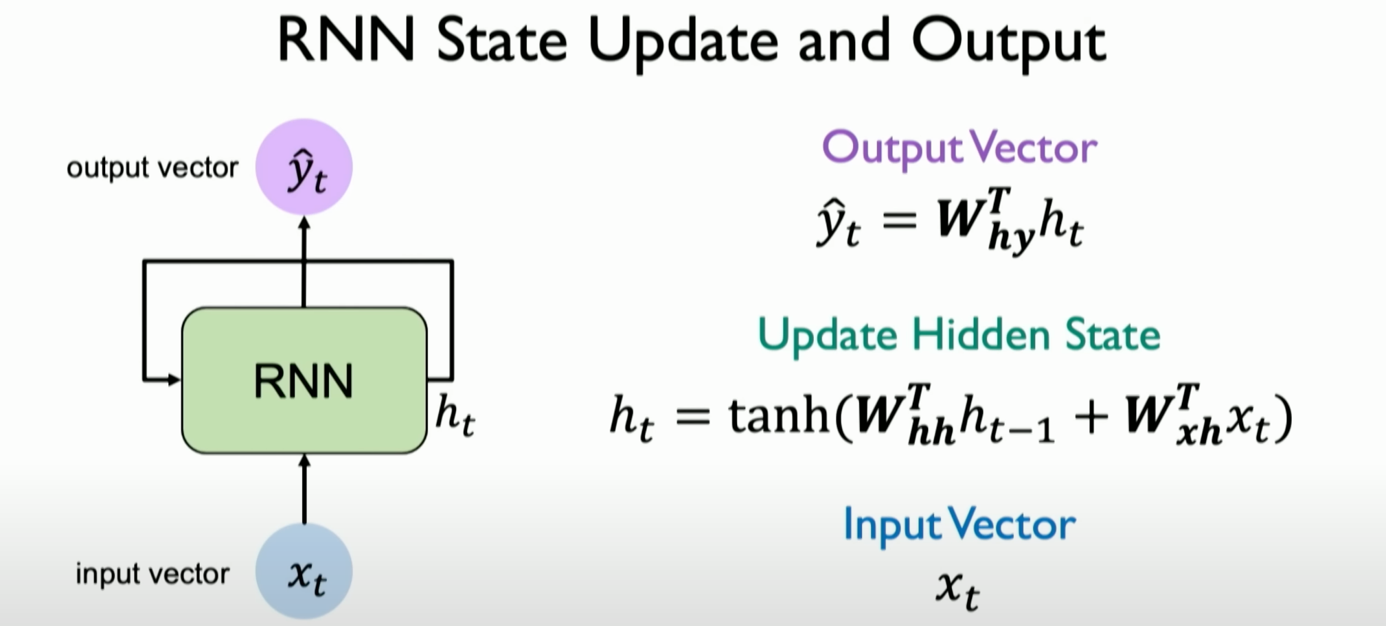
We understand the internal state’s update process through a mathematical description. At each time step, we calculate the internal state using a new function W that takes the current time step’s inputs X of t and the previous internal state as inputs.
RNN Intuition
- Recurrence Concept: The instructor introduces the concept of recurrence by comparing it with traditional perceptrons. In perceptrons, inputs are treated as independent and not part of a sequence. In RNNs, inputs are viewed as part of a sequence, and the network’s output depends on both current input and previous inputs.
- Time Steps and States: RNNs consider time steps when processing data. The instructor notes that each operation in RNNs is based on the current input and the internal state (or memory) from previous time steps.
- State Update: RNNs use recurrence relations to maintain and update their internal state. This relation defines how the computation at a specific time step affects subsequent time steps.
- RNN Implementation: The instructor introduces how to implement RNNs, including defining RNNs in Python code, initializing hidden states, and processing input sequences.
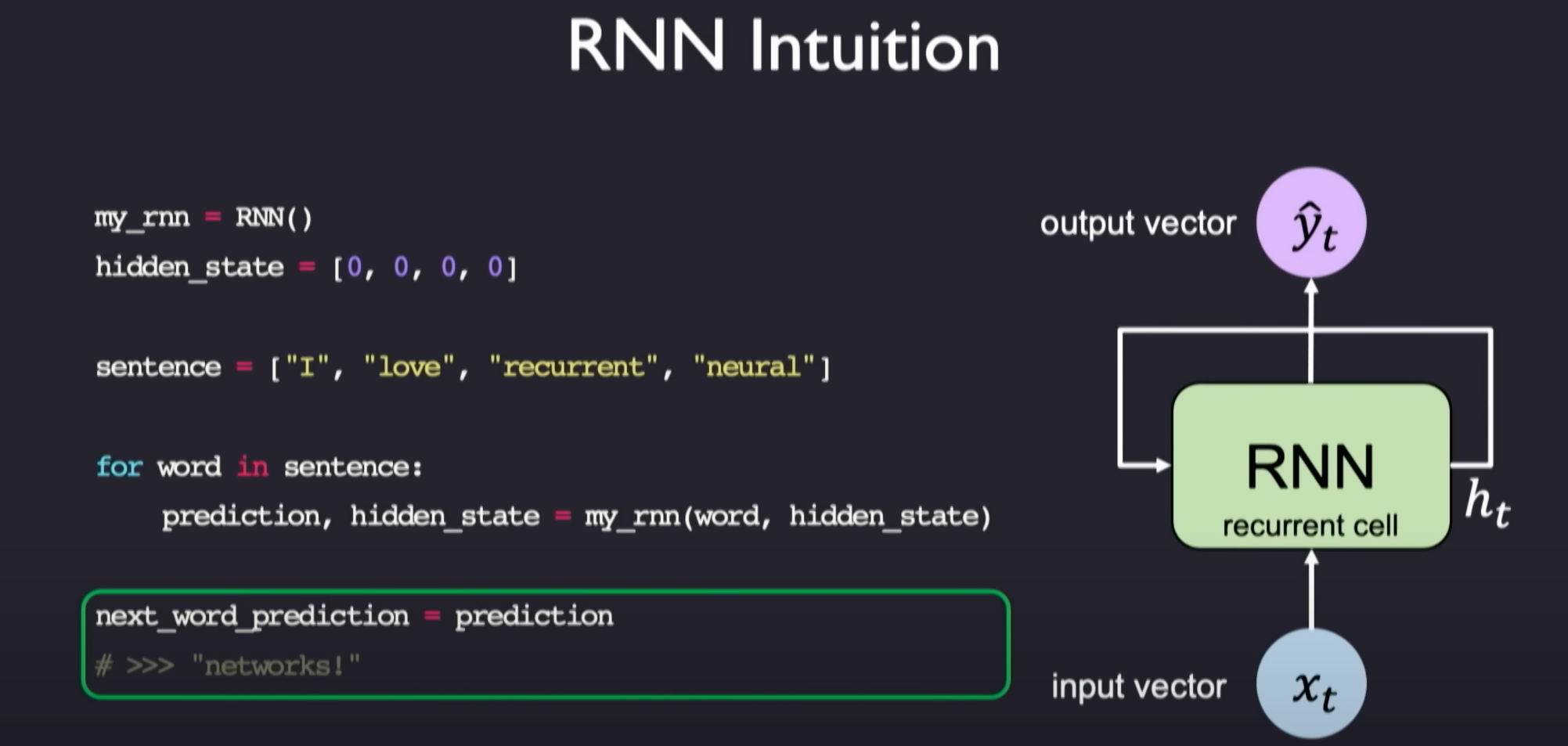
1 | # Create an RNN instance |
Above is the pseudocode to implement this process.
Unfolding RNNs
We can see that the computation of RNNs includes updating the hidden state and generating some predicted output, which is our final goal of interest.
The basic computation process of Recurrent Neural Networks (RNNs) can be divided into the following steps:
Initialization of Input and Hidden States: RNNs begin by initializing the input data and hidden states. The input data is typically sequential data, such as a series of words or time-series data. Hidden states are the mechanism by which RNNs remember previous inputs, generally initialized to zero or a small random number.
Processing Each Time Step: For each element in the sequence (e.g., each word in a sentence), RNNs perform a series of computations involving the current input and the hidden state from the previous time step.
a. Input Processing: The input data of the current time step is processed. If the input data is non-numeric, like text, it first needs to be converted into a numeric form, usually a vector (e.g., through word embeddings).
b. Hidden Layer Computation: RNNs update their hidden state by combining the current time step’s input with the hidden state from the previous time step. This typically involves one or
more linear transformations (weighted sums) and a non-linear activation function. The formula is usually: tanh or ReLU.
c. **Output Prediction**: Based on the updated hidden state, RNNs compute the current time step's output, which may include linear transformations and activation functions. In some applications (like language models), the output might be a prediction of the next element in the sequence. The formula can be $ y_t = W_{hy}^ {T} h_t + b_y $, where $ y_t $ is the output.
Sequence Processing: The above steps are repeated for each element in the sequence until the entire sequence is processed.
Output Sequence: Depending on the application, RNNs can output either the final time step’s output or the entire sequence’s output.
Error Backpropagation and Parameter Update: During training, RNNs calculate the error between the output and the actual values and update the network’s weights using the backpropagation algorithm to minimize this error.
RNNs are particularly suitable for handling sequential data because they can capture the time dynamics in the sequence. However, traditional RNNs face issues like vanishing and exploding gradients, limiting their effectiveness in handling long sequences. To address this, more complex RNN variants, such as Long Short-Term Memory (LSTM) networks and Gated Recurrent Units (GRUs), have been developed.
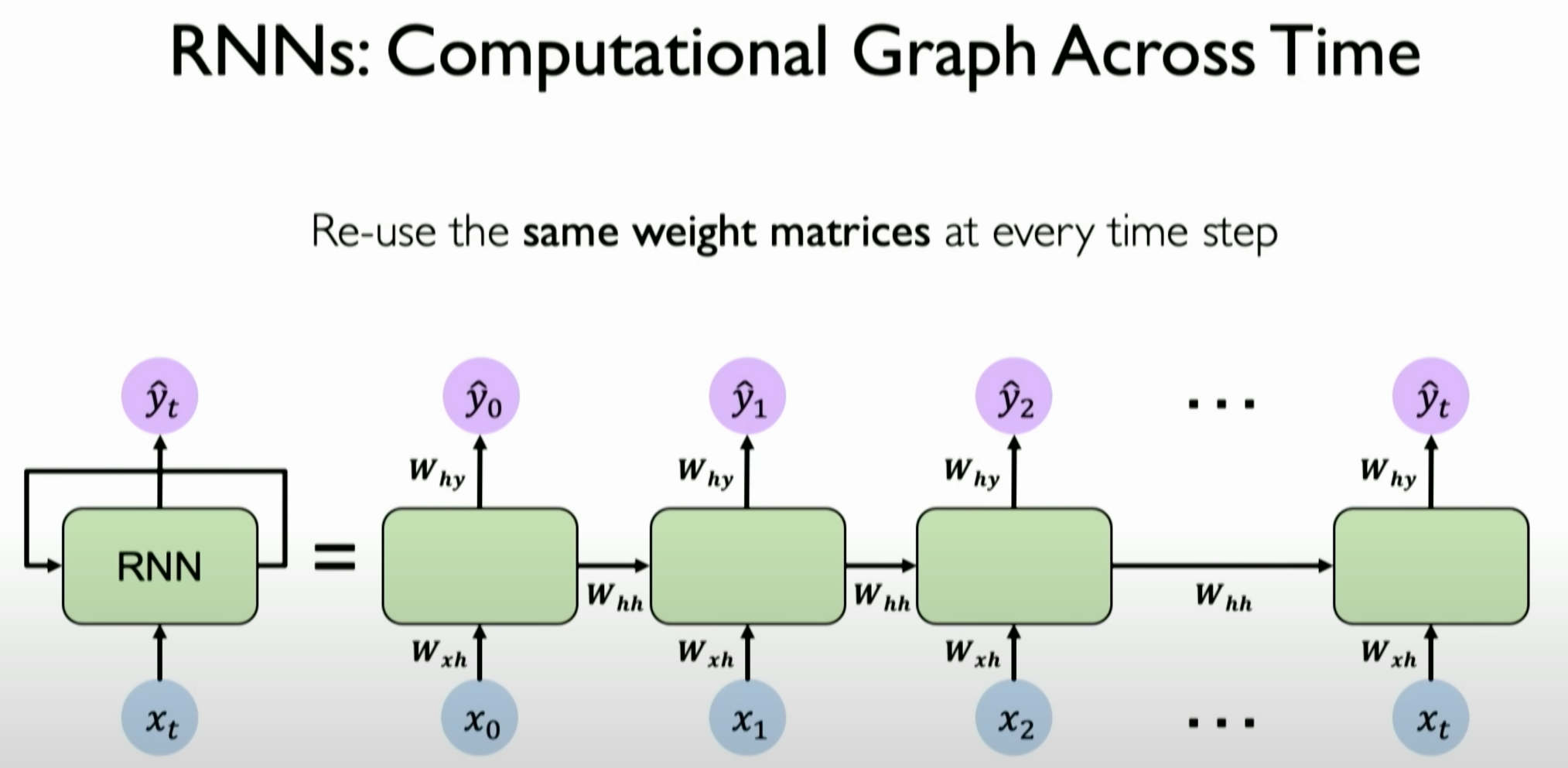
RNNs can be represented as a recursively reused network, where the same three weight matrices are reused at each independent time step to operate on input data and hidden states, generating new hidden states and outputs. These three sets of weight matrices are:
Input to Hidden State Weight Matrix
: - This matrix processes the current time step’s input data.
- It transforms input data into a form matching the hidden layer size.
- At each time step, the current input
is multiplied by this matrix, forming part of the contribution to the hidden state.
Hidden State to Hidden State Weight Matrix
: - This matrix processes the previous time step’s hidden state.
- It defines how to update the current hidden state based on the previous time step’s hidden state
. - This matrix is crucial for RNNs to “remember” the sequence history.
Hidden State to Output Weight Matrix
: - This matrix generates output based on the current hidden state.
- It transforms the hidden state into the final output, such as the probability distribution of the next word in a language model.
- This matrix determines how the current hidden state affects the output result.
At each time step, RNNs use these matrices to generate outputs and update hidden states:
- First, the current input
is multiplied by . - Simultaneously, the previous time step’s hidden state
is multiplied by . - These results are added and passed through an activation function (e.g.,
tanhorReLU) to produce the new hidden state. - The new hidden state
can generate output by multiplying it with .
This mechanism of reusing weight matrices is the basis for RNNs to handle sequential data, allowing the network to transmit information over time and make decisions based on past information.
RNNs from Scratch
The process of training Recurrent Neural Networks (RNNs) and defining the loss involves several key steps:
1. Initializing Weight Matrices and Hidden State
- Weight Matrices: Initialize the weight matrices used in RNNs for input to hidden state, hidden state to hidden state, and hidden state to output.
- Hidden State: Usually initialized to zero. This is the mechanism by which RNNs retain past information, updating it with each time step’s input.
2. Forward Propagation
- At each time step, RNNs receive an input (
) and update the hidden state ( ). - The hidden state update is based on the current input and the hidden state from the previous time step.
- The updated hidden state generates the current time step’s output.
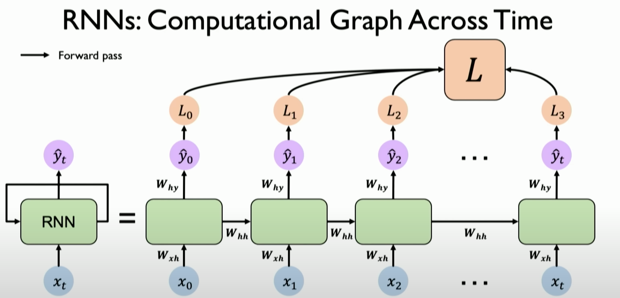
3. Loss Calculation
- At each time step, the output of the RNN is compared with the actual labels, and the loss for that time step
is calculated. - For sequence generation tasks (e.g., language models), the cross-entropy loss function is commonly used.
- For sequence classification tasks, the loss may only be calculated at the final time step’s output.
- The total loss
is the accumulation of all time steps’ losses.
4. Backpropagation and Weight Update
- Using the backpropagation algorithm (e.g., gradient descent), update the weight matrices based on the total loss.
- During backpropagation, the error signals are propagated from the output layer back to the input layer through each time step’s hidden state.
5. Iterative Training
- Repeat the steps of forward propagation, loss calculation, backpropagation, and weight update until the model achieves satisfactory performance.
Implementation Example
From scratch definition: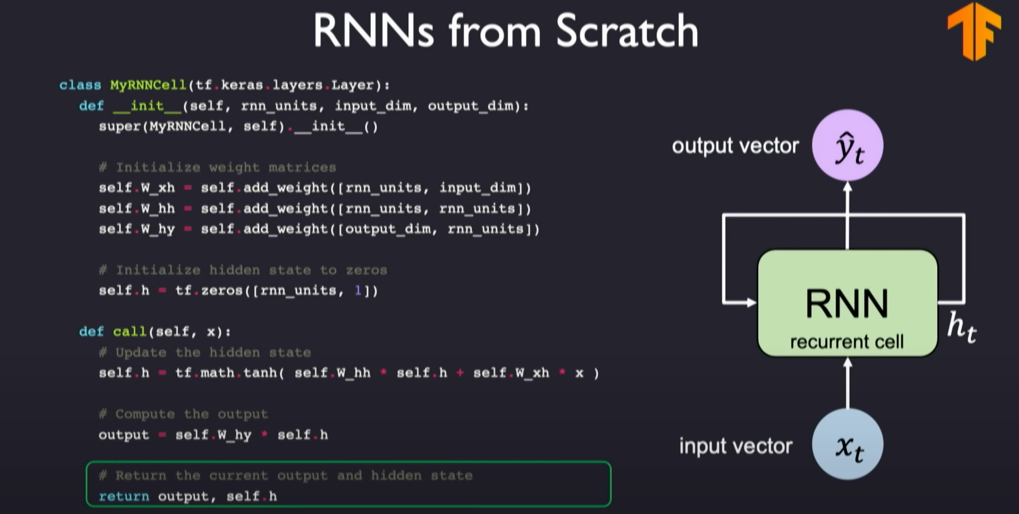
1 | import tensorflow as tf |
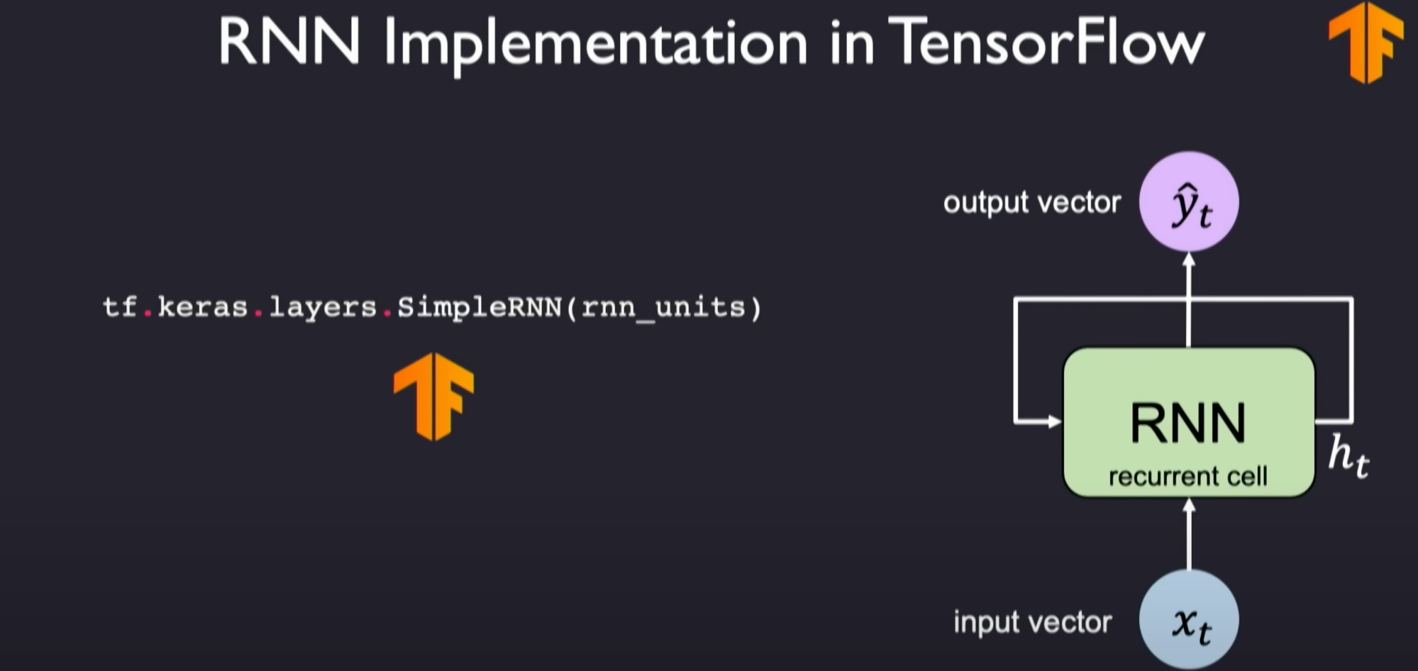
TensorFlow provides abstract APIs for implementation, making it easy to call APIs to implement your own RNN.
When implementing RNNs in TensorFlow, you can define an RNN layer class. This class includes methods for initializing weight matrices, updating hidden states, and generating outputs based on hidden states. This process is repeated for each time step to process the entire input sequence.
1 | import tensorflow as tf |
In this example, the SimpleRNNLayer class handles the operations for a single time step, while the SimpleRNNModel class manages the processing of the entire sequence. This model can be trained and optimized for specific tasks.
Design Criteria for Sequential Modeling
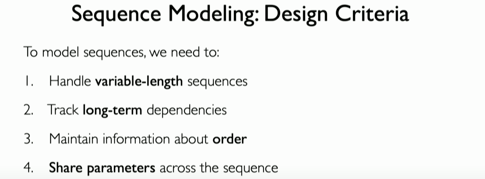
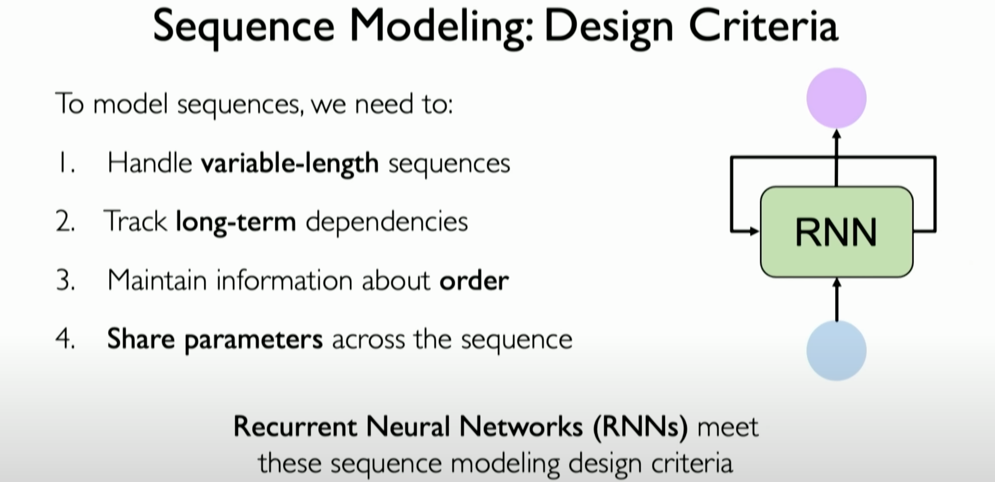
When dealing with sequential modeling problems, RNNs need to meet the following four design criteria:
Handling Variable-Length Sequences: The RNN model should handle sequences of different lengths, meaning the model should be effective whether the sequences are short or long.
Tracking and Learning Temporal Dependencies: A key task of RNNs is to track and learn dependencies that develop over time in the data. This may include dependencies between elements that are far apart in time.
3
. Maintaining Order Information: A fundamental characteristic of sequence data is that the current input depends on the specific order of previous inputs. RNNs need to maintain this order information as it has a significant impact on the final prediction results.
- Parameter Sharing: RNNs need to implement parameter sharing, meaning the same set of weights should be applied across different time steps in the sequence to generate meaningful predictions. This helps the model maintain consistency and effectiveness when handling data at various time steps.
These design criteria ensure that RNNs effectively handle sequential data and drive the research and development of more robust architectures that may outperform RNNs in sequential modeling.
Word Prediction Example
Problem Description: Given a series of words, the task is to predict the next word in the sentence. For example, given the sentence “This morning I took my cat for a walk,” the task is to predict the final word in the sentence.
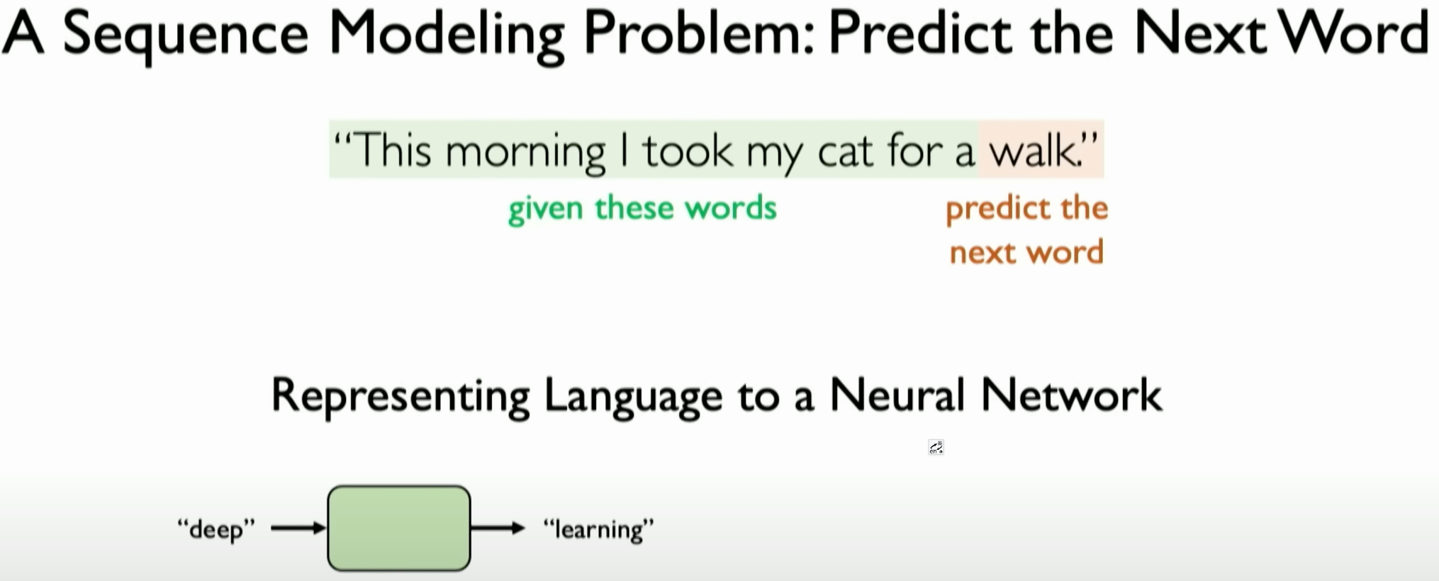
Converting Language Information into Numerical Encoding: Before defining the RNN, determine how to convert textual information into numerical encoding that a neural network can process and understand. Neural networks cannot directly process language; they operate on mathematical functions.
Concept of Embedding: The key method for converting language information into numerical encoding is through “embedding.” This involves mapping each word in the vocabulary to a fixed-size numerical vector. A common approach is defining all possible words in the vocabulary and assigning a unique index label to each word, creating a so-called “one-hot” embedding vector.
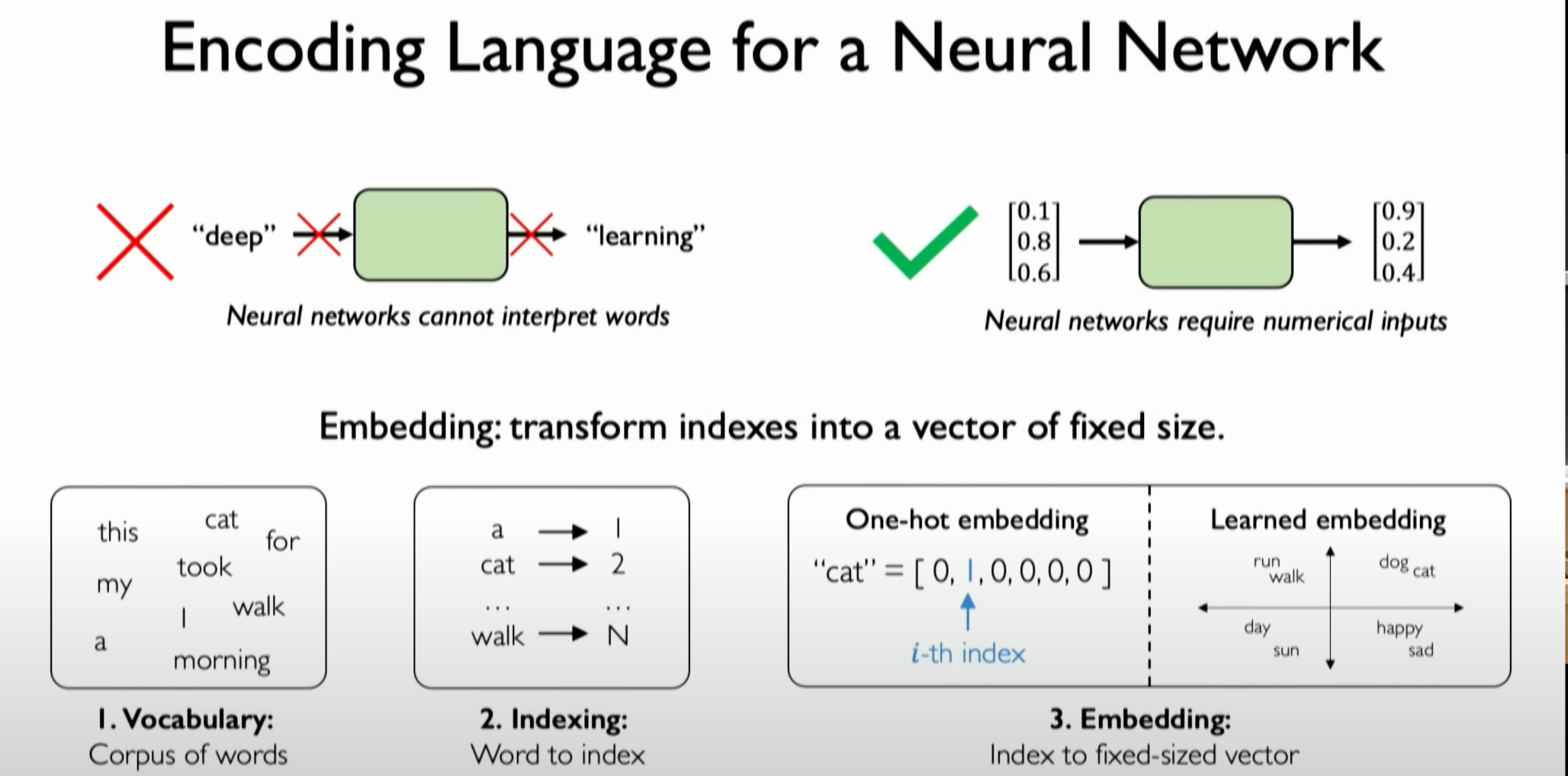
Learning Embeddings with Neural Networks: Another approach is using neural networks to learn embeddings, capturing the inherent meaning or semantics in the input data, and making related words or inputs more closely linked in the embedding space.
Design Criteria: When handling such problems, RNNs need to meet several key criteria: handling variable-length sequences, tracking dependencies in sequence data, maintaining order information, and applying the concept of parameter sharing.
Overall, this section delves into how to use RNNs to process and predict sequence-based text data, emphasizing the importance of embedding techniques and key considerations when designing and training RNNs.
Backpropagation Through Time
Backpropagation Algorithm: The backpropagation algorithm is a key technique for training the weights in Recurrent Neural Networks (RNNs). This algorithm is an extension of the standard backpropagation algorithm for handling sequential information.
Process of Backpropagation: In feedforward neural networks, the backpropagation algorithm typically involves forward passing the input through the network, comparing the predicted result with the actual result to calculate the loss, and then backpropagating the loss through the network to update the weights. In RNNs, this process needs to be adjusted for sequential data.
Phase 1: Propagation of Excitation- Forward Propagation Phase: In BPTT, this step involves passing the entire input sequence (rather than a single input) through the RNN. The network processes the input at each time step and produces the corresponding output. During this process, the network maintains and updates its internal state (hidden state), which captures information from previous steps in the sequence.
- Backward Propagation Phase: At each time step of the sequence, the network’s predicted results are compared with the actual targets, and the loss is calculated. Unlike standard BP, the loss here is calculated at each time step of the sequence, not just a single output.
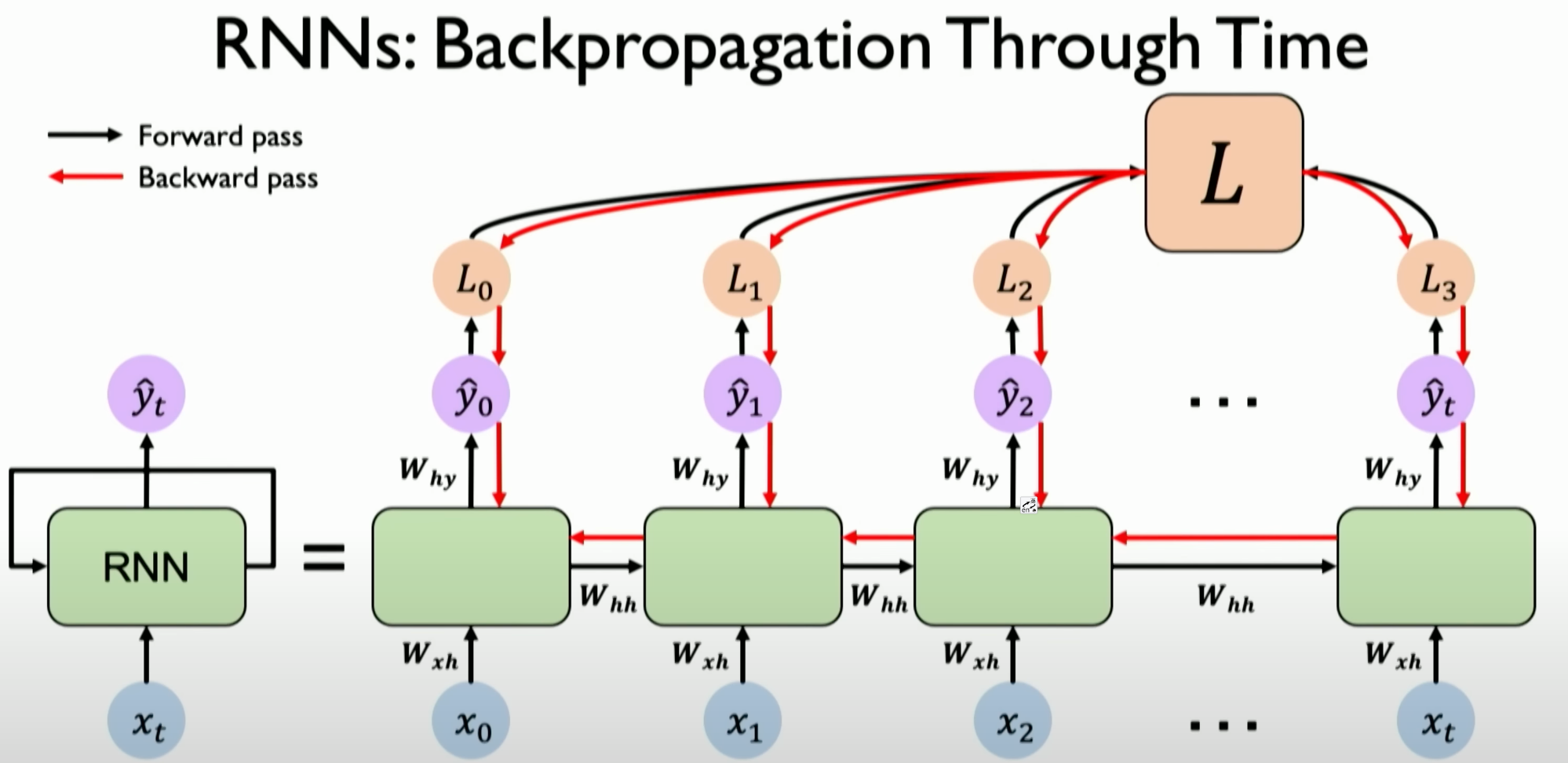
Phase 2: Weight Update- In BPTT, the process of updating weights is similar to the standard BP algorithm but with some differences. First, the calculated gradient depends not only on the error at the current time step but also on errors from previous time steps. This is because the current state of the RNN is based on all previous states.
- The gradient for each weight is obtained by multiplying the input excitation (in this case, the input and hidden states from the current and previous time steps) with the response error. This gradient is then used to update the network weights, typically by multiplying by a learning rate (i.e., the “training factor”) and taking the negative.
Iterative Process- In BPTT, this iterative process involves the entire sequence. The network needs to forward and backward propagate at each time step of the sequence until the entire sequence’s output achieves satisfactory results. This means BPTT needs to handle longer dependencies, making it computationally more complex and challenging.
In summary, BPTT is conceptually similar to the standard BP algorithm but is designed specifically to handle sequential data and the characteristics of RNNs, such as continuous state updates and dependencies between time steps. This makes BPTT more complex to implement and execute than the standard BP algorithm.
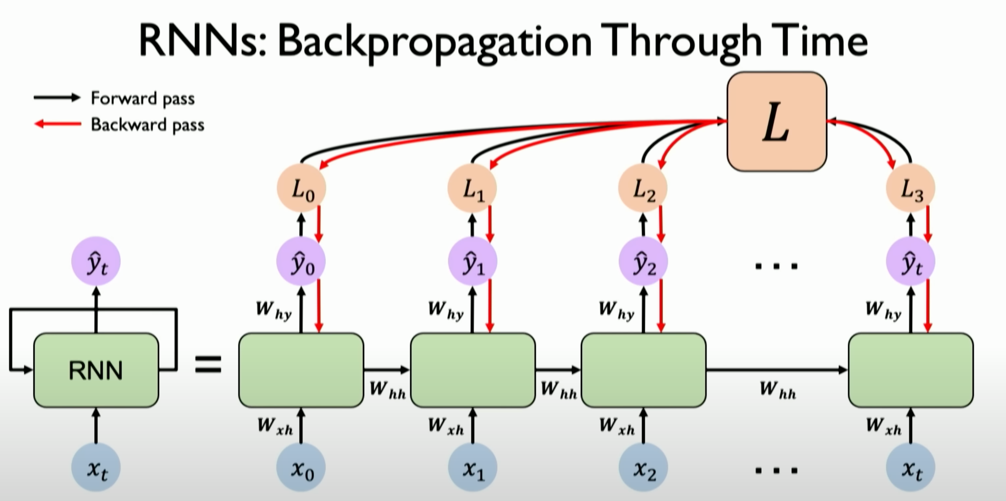
First, backpropagate the loss through each individual time step.
Then, perform backpropagation operations across all time steps, from the current time
Tback to the beginning of the sequence. This is why the algorithm is called Backpropagation through Time.Because data and predictions and the resulting errors provide timely feedback from our current position all the way to the beginning of the input data sequence.
Unfolding in Time: In RNNs, because the output of each time step depends on the current input and previous hidden states, when computing gradients, the entire input sequence needs to be considered. This requires unrolling the RNN in time to track and update the states and gradients for each time step.
Loss Calculation and Weight Update: In RNNs, the loss at each time step needs to be calculated and accumulated to form the total loss. This total loss is then used to backpropagate through each time step of the sequence to update the network’s weights.
Gradient Issues
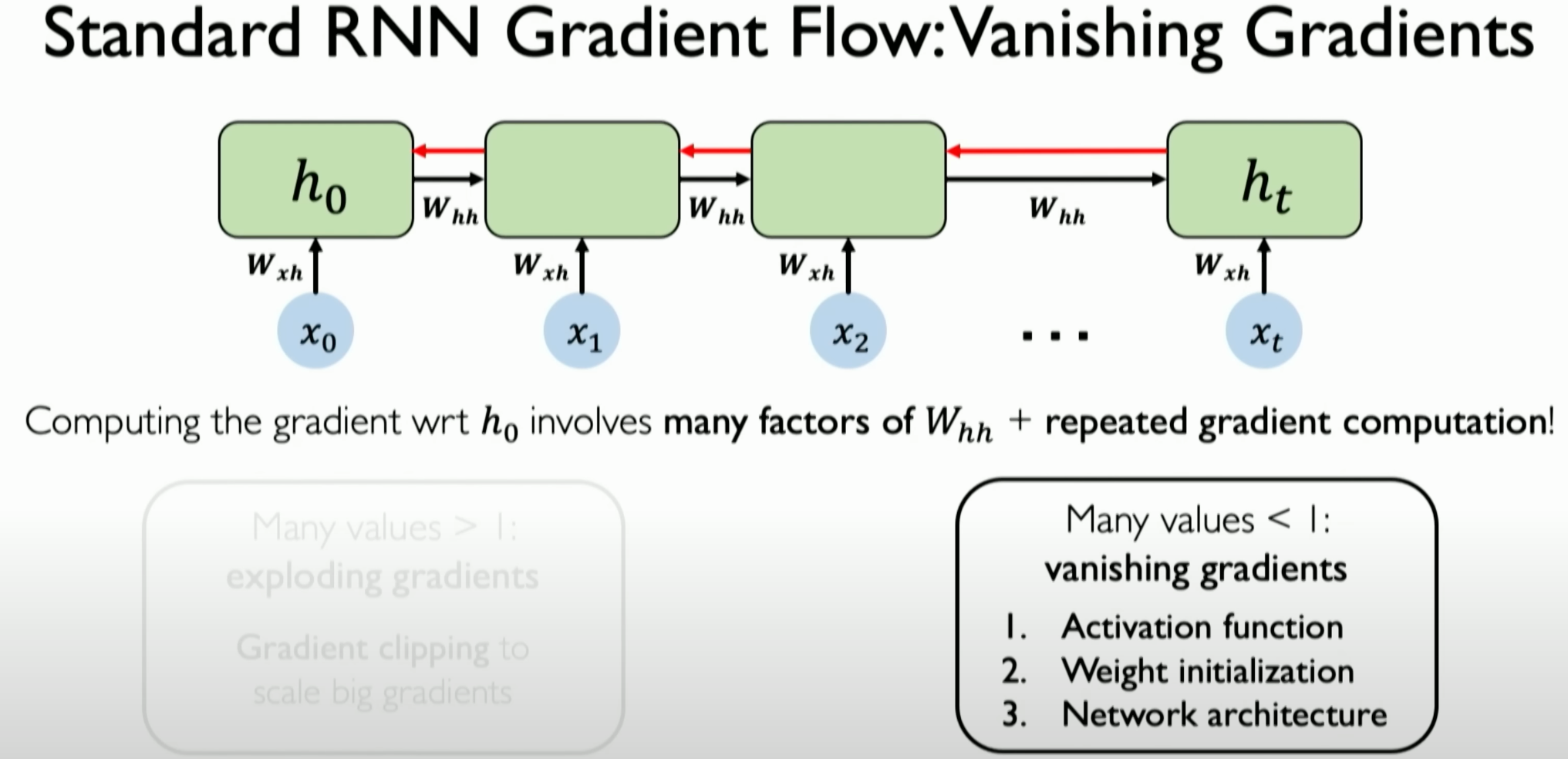
Recurrent Neural Networks (RNNs) face two major gradient issues: exploding gradients and vanishing gradients.
Exploding Gradient Problem:
- Exploding gradients refer to the situation where the gradients become excessively large during the training process of RNNs, making it unstable to train the network. This problem usually occurs when the weight matrix
is large, causing the gradients to increase dramatically during backpropagation through the network. - To solve the exploding gradient problem, a method called “gradient clipping” can be employed. This method limits the gradient size to keep it within a reasonable range, preventing the gradient values from becoming too large.
- Exploding gradients refer to the situation where the gradients become excessively large during the training process of RNNs, making it unstable to train the network. This problem usually occurs when the weight matrix
Vanishing Gradient Problem:
- Vanishing gradients refer to the situation where the gradients become extremely small, nearly zero, during the training process of RNNs, making it difficult for the network to learn and update weights. This problem usually occurs when the weight matrix
is small, causing the gradients to diminish to nearly zero during backpropagation through the network. - The vanishing gradient problem is particularly important for RNNs because it can prevent RNNs from learning long-term dependencies in the input sequence.
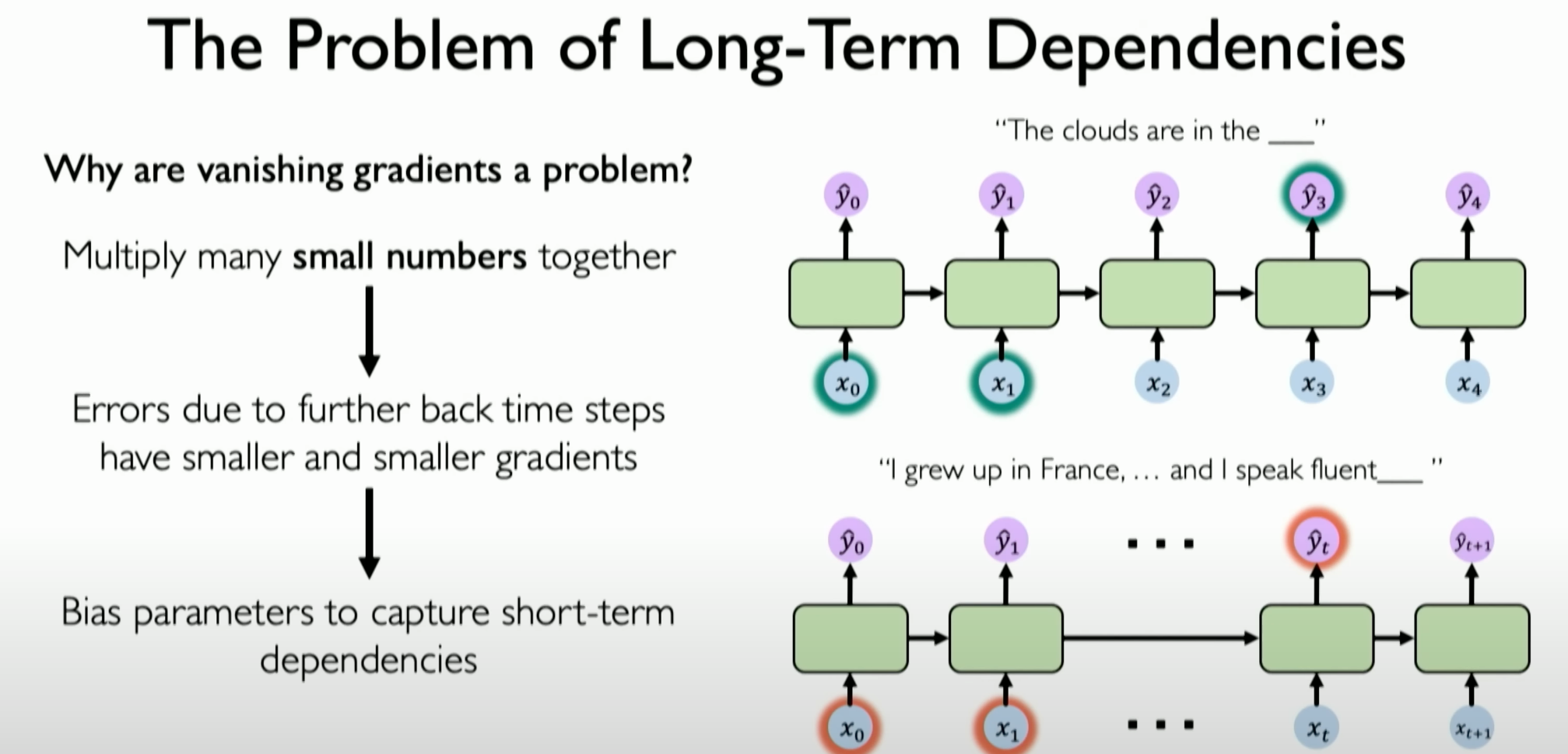
We can illustrate the vanishing gradient problem with a simple example. When dealing with short sequences, the distances between time steps in RNNs are short, meaning the network only needs to learn and maintain short-term dependencies. For example, consider the simple sequence “I am hungry, so I ate an apple.”
In this case, since the sequence is short, the association between the current word (e.g., “apple”) and the previous word (e.g., “ate”) is easily captured. The gradients can flow effectively since they do not need to backpropagate through too many time steps.
Therefore, in short sequences, the vanishing gradient problem is not as apparent, and the network can effectively learn the dependencies in the sequence.
When dealing with ultra-long sequences, such as a text containing hundreds of words, RNNs need to learn and maintain dependencies spanning a longer range of time steps. This may include context relationships that span an entire paragraph.
In this case, since the sequence is too long, the gradients need to backpropagate through more time steps. As gradients pass through each time step during backpropagation, they may gradually diminish, especially if using traditional activation functions (e.g., tanh or sigmoid).
This leads to gradients in earlier time steps of the network becoming very small, nearly zero, making it difficult for the network to learn and maintain important information from early time steps in the sequence. As a result, even though the network may perform well in handling recent information in the sequence, it cannot effectively learn and remember
- Vanishing gradients refer to the situation where the gradients become extremely small, nearly zero, during the training process of RNNs, making it difficult for the network to learn and update weights. This problem usually occurs when the weight matrix
long-term dependencies.
Three Techniques to Address Vanishing Gradients
Three techniques to address the vanishing gradient problem can be summarized as follows:
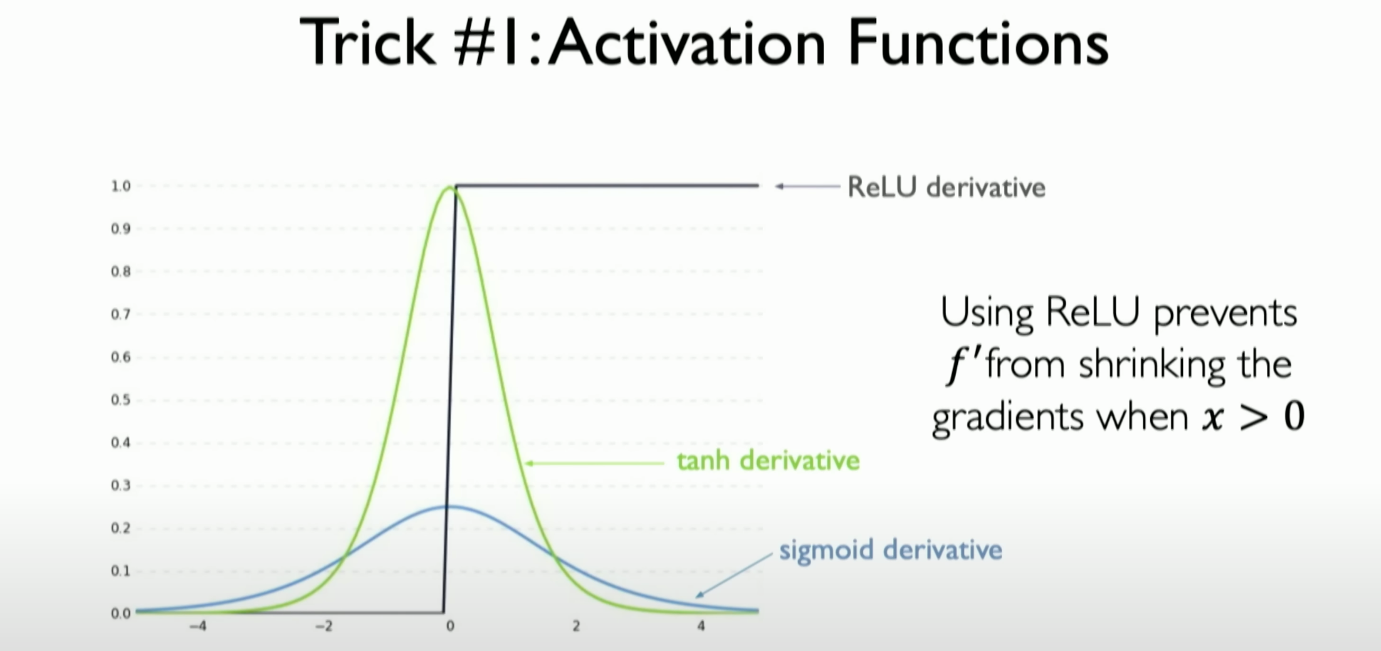
Change Activation Functions:
Changing the activation functions in each layer of the neural network, especially using the ReLU (Rectified Linear Unit) activation function. The advantage of ReLU is that its derivative is 1 when the input is greater than zero, preventing the gradient from vanishing in the positive input region. This helps maintain larger gradients in the positive data region, alleviating the vanishing gradient problem.
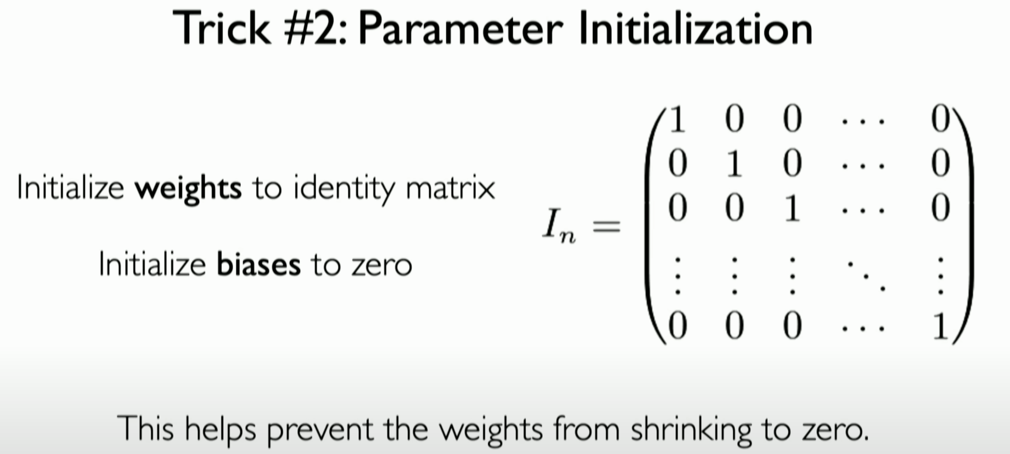
Parameter Initialization Methods:
Improving the initialization of parameters in neural networks, such as initializing weights as Identity matrices. Such initialization helps prevent weights from rapidly shrinking to zero during the early stages of training. Proper parameter initialization ensures stable gradient flow during the early stages of training, preventing gradients from vanishing too early.
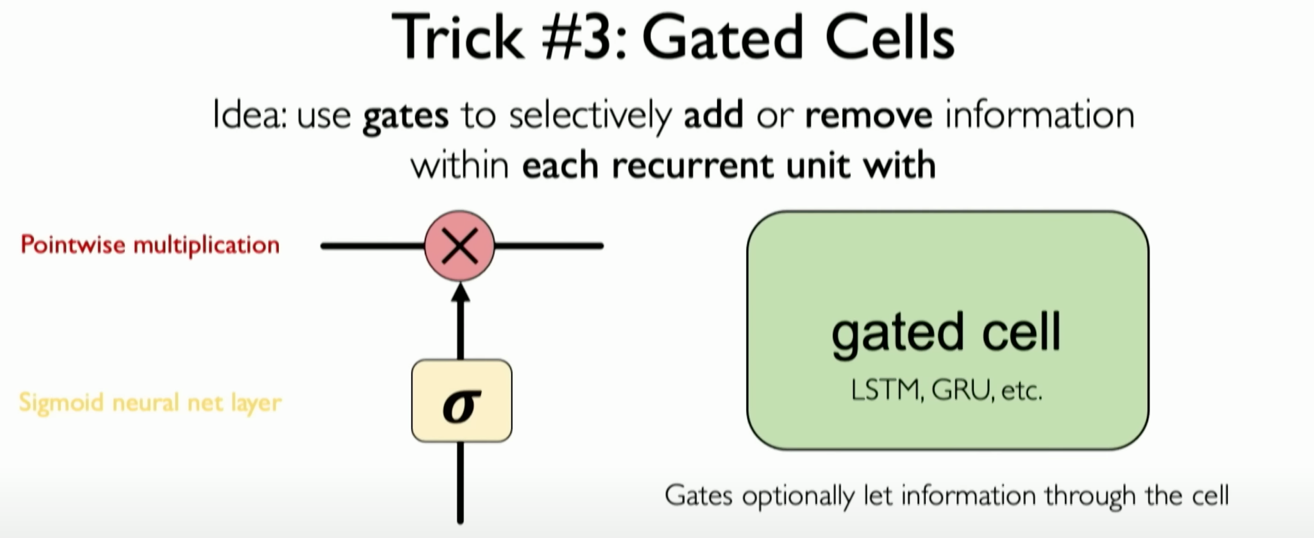
Introducing Gated RNN Variants:
Using Long Short-Term Memory (LSTM) or other RNN variants with gating mechanisms. LSTMs use various gates (such as forget gate, input gate, and output gate) to control the flow of information, effectively filtering and storing important information. This gating mechanism allows the network to maintain and update an independent cell state, helping to maintain gradient flow throughout the sequence, significantly mitigating the vanishing gradient problem.
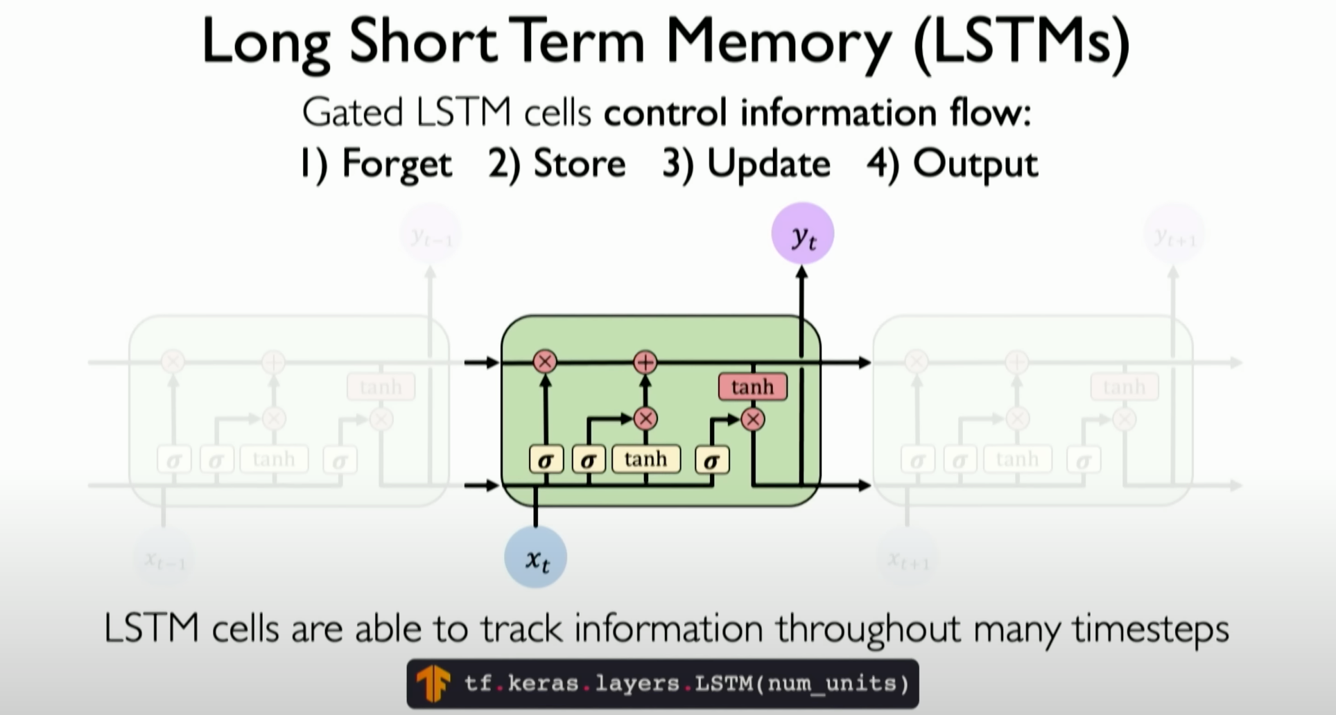
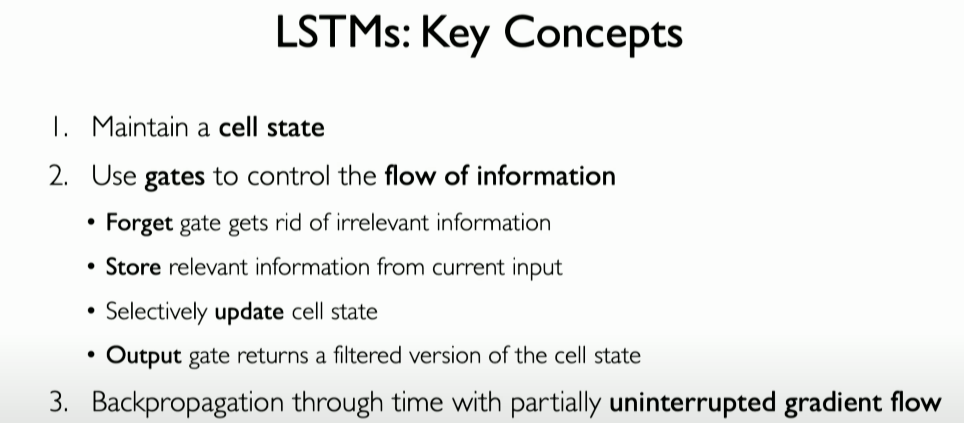
Long Short-Term Memory networks (LSTMs) are a special type of Recurrent Neural Network (RNN) specifically designed to address the vanishing and exploding gradient problems when dealing with long sequential data. The key feature of LSTMs is their gating mechanism, which allows them to effectively learn long-term dependencies. The main components and workings of LSTMs are as follows:
Forget Gate:
The forget gate decides which information should be discarded or retained from the cell state. It operates through a sigmoid layer that examines the current input and the previous time step’s hidden state, outputting a value between 0 and 1. Values close to 0 mean the information should be discarded, while values close to 1 mean the information should be retained.
Input Gate:
The input gate comprises two parts: a sigmoid layer and a tanh layer. The sigmoid layer decides which values will be updated, while the tanh layer creates a new candidate value vector that can be added to the state.
Cell State:
The cell state is the core of LSTMs, running through the entire chain with only minor linear interactions. It can carry relevant information across long distances, retaining long-term dependencies. The cell state is updated by the forget gate, deciding which old information to discard, and by the input gate, adding new information.
Output Gate:
The output gate decides the value of the next hidden state, which contains information about the current time step’s output. The hidden state is also used to predict the next time step’s output. The output gate examines the current cell state and determines which information will be used as output.
The gating mechanisms of LSTMs work together, allowing the network to automatically learn when to forget old information and when to introduce new information, greatly improving the model’s performance and stability when handling long sequential data. Consequently, LSTMs perform exceptionally well in tasks involving long-term dependencies, such as language modeling, machine translation, and speech recognition.
These three methods each have their advantages, effectively addressing or at least mitigating the vanishing gradient problem, and improving the performance and stability of recurrent neural networks when handling long sequential data.
RNN Applications
Here, we introduce two specific examples of applications of Recurrent Neural Networks (RNNs) in various fields, demonstrating their practical uses in different domains:
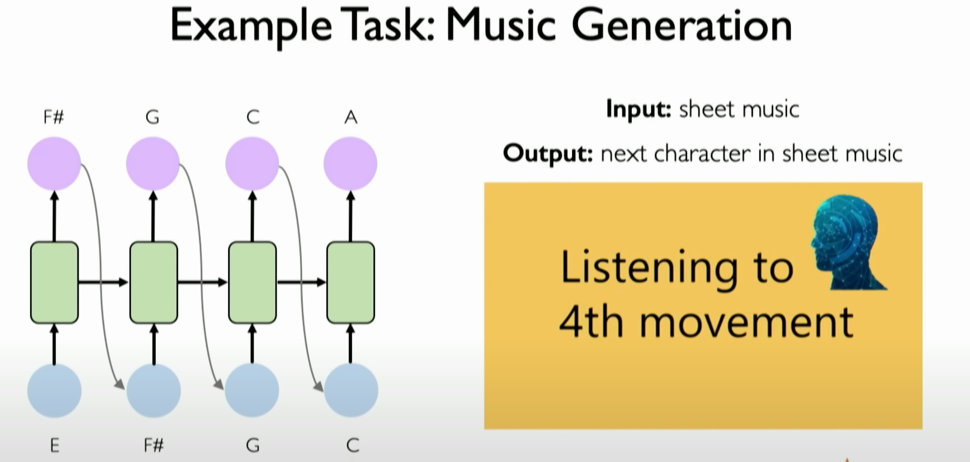
Music Generation:
- RNNs can be used for music generation, where the task is to build an RNN to predict the next note in a music sequence. This application can be used to generate entirely new music sequences that have never been created before.
- A specific example is a few years ago when a team used an RNN-based model to attempt to generate the third movement of composer Schubert’s unfinished symphony. Schubert’s symphony was only completed for two movements, and he died before completing the third movement. The music results generated using RNN demonstrated the potential of RNN in music creation.
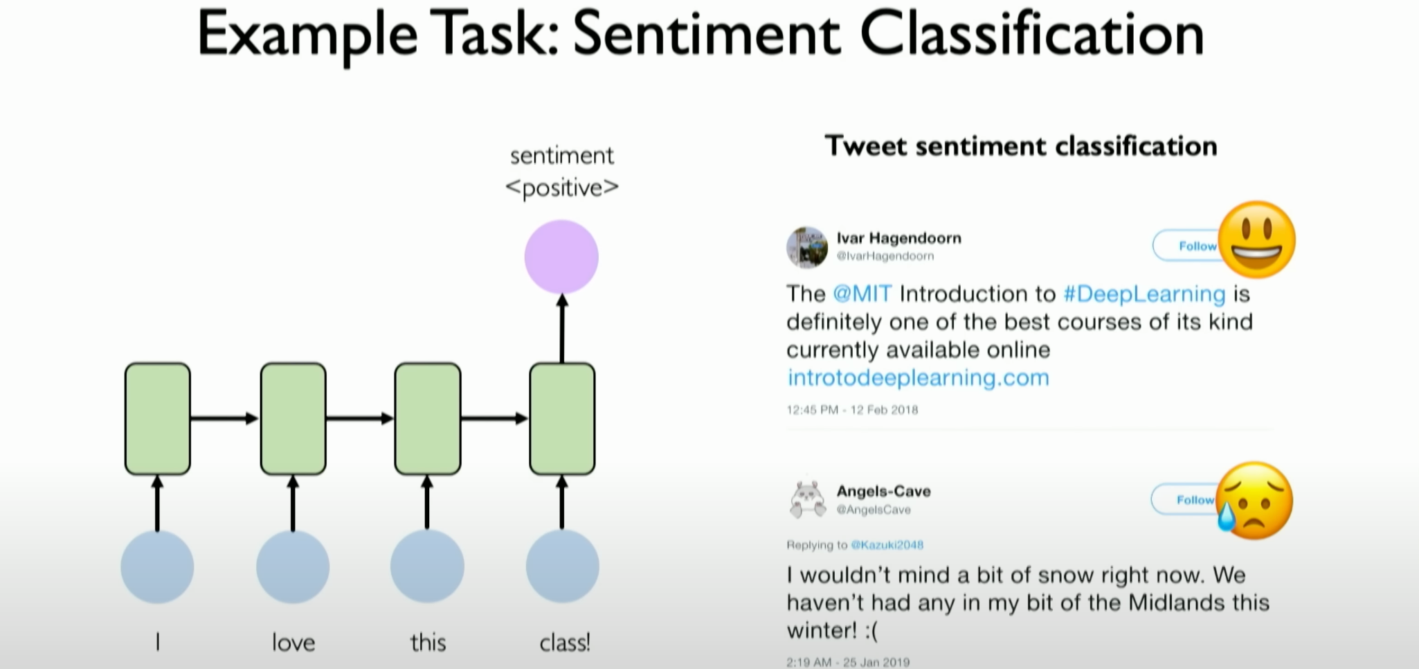
Sentiment Classification:
- RNNs can also be applied to sentiment classification tasks, such as processing text data (e.g., tweets) and assigning positive or negative labels to the text based on its content. This application leverages the RNN’s ability to handle sequential data, extracting sentiment information from the text and classifying it accordingly.
- In this context, RNNs can understand and analyze the emotion or sentiment tendency in the text, such as determining whether a tweet expresses positive or negative sentiment.
These application examples show that RNNs are well-suited for tasks involving sequential data, making them ideal for fields such as music generation and sentiment classification. The diversity and practical effectiveness of these applications highlight the powerful capabilities of RNNs in handling sequential data.
Limitations of Recurrent Models
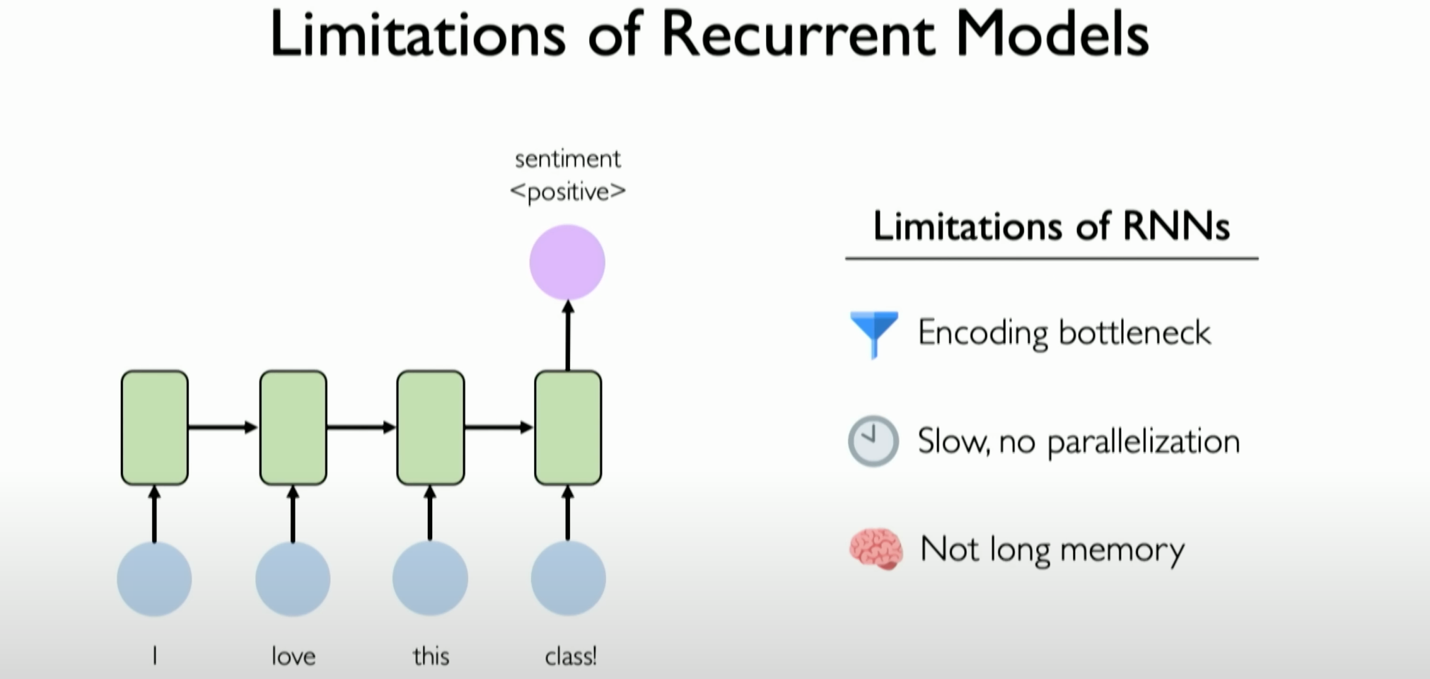
Recurrent Neural Networks (RNNs) and their variants, such as Long Short-Term Memory (LSTM) networks, although effective in handling sequential data, have several limitations. The main limitations of RNNs are as follows:
Encoding Bottleneck:
- RNNs need to process and handle information step by step when dealing with sequential data. This leads to an “encoding bottleneck,” where attempting to encode a large amount of content (e.g., a long text) into a single output may only occur at the last time step of the sequence.
- In practice, ensuring all information leading to that time step is correctly maintained and encoded is challenging, and much information may be lost.
Slow Processing Speed (No Parallelization):
- Since RNNs process data step by step, their processing speed may be relatively slow. This step-by-step processing method of RNNs does not allow for simple parallelization, limiting their efficiency when dealing with large datasets.
Limited Long-Term Memory:
- Although LSTMs are designed to address the vanishing gradient problem in handling long-term dependencies, in practice, the ability of RNNs and LSTMs to handle long-term dependencies remains limited. RNNs and LSTMs struggle to effectively handle long sequences containing tens of thousands or more time steps, affecting their ability to learn and maintain all information and patterns in those sequences.
Overall, while RNNs and LSTMs excel in handling sequential data, they still have limitations in encoding bottlenecks, processing speed, and long-term memory capabilities. These limitations drive researchers to develop new architectures and methods, such as Transformers, to more effectively handle sequential data.
Attention Fundamentals
The limitations of Recurrent Neural Networks (RNNs) have been previously mentioned. Due to step-by-step processing in each time step, this leads to three fatal issues, necessitating the establishment of a new architecture capable of continuously processing information flow.
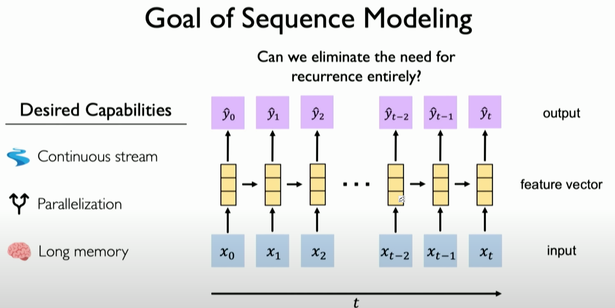
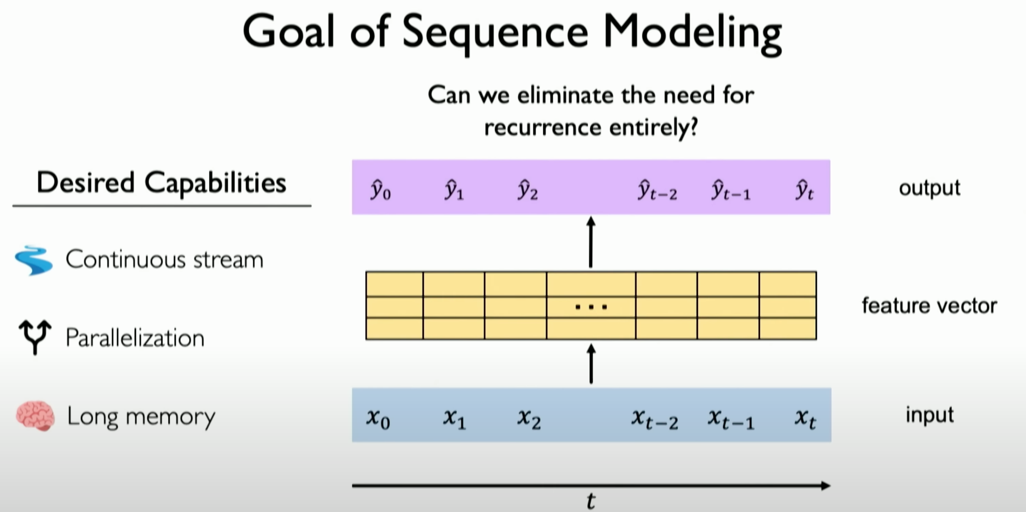
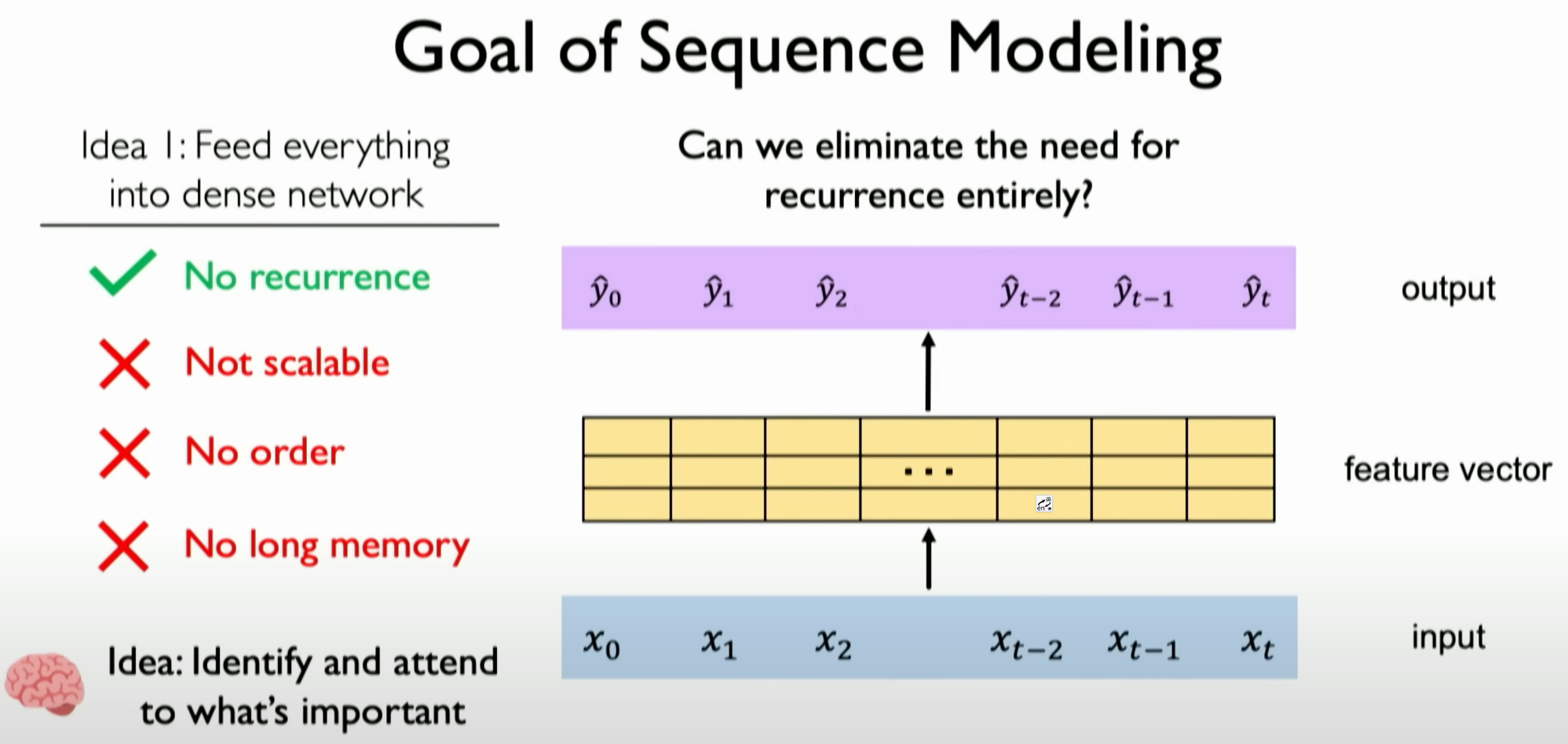
Need Beyond RNNs
- To address these issues, researchers sought to establish an architecture capable of continuously processing information flow, rather than step-by-step processing.
- The goal is to create a scalable architecture while maintaining the order and time dependencies in the data and building more robust long-term memory capabilities.
Intuition of Attention
The attention mechanism was proposed to address the key limitations of Recurrent Neural Networks (RNNs) in sequential data
processing, particularly encoding bottlenecks, slow processing speed, and limited long-term memory capabilities. By introducing a mechanism that allows the model to effectively process the entire data sequence in parallel rather than step by step, it enables the network to focus on important parts of the input and build a more detailed and rich understanding of sequential data.
Introduction of the Attention Mechanism
- Attention or Self-Attention mechanisms were introduced to identify and focus on important information in sequential data.
- This mechanism allows the model to recognize and focus on important elements in a potential sequence information flow, a highly powerful concept in modern deep learning and artificial intelligence.
- Through the attention mechanism, the model can more effectively extract information from the input data while preserving the order of the sequence.
Impact of the Attention Mechanism
- The introduction of the attention mechanism marks a shift from step-by-step recurrent processing to more flexible and powerful data processing architectures.
- It opens new possibilities for handling complex and long-sequential data, transforming traditional approaches in fields like computer vision and language models.
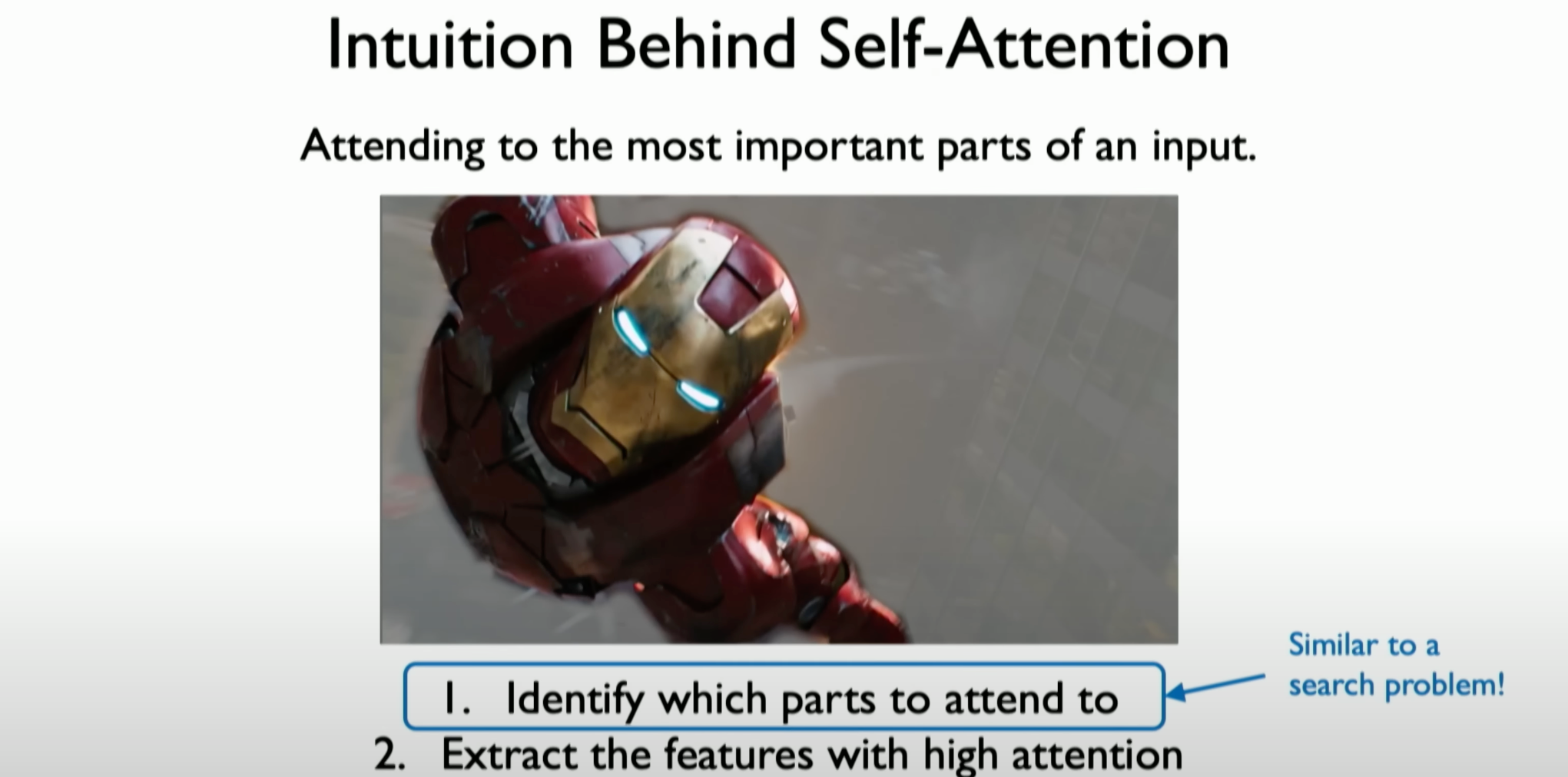
We can intuitively introduce the self-attention mechanism using an image of Iron Man. When we look at an image of Iron Man, we do not analyze the entire image pixel by pixel (similar to step-by-step processing); instead, we directly focus on important parts, such as Iron Man’s face and body. This process reflects a type of calculation possibly happening in our brain. The key is how the brain identifies and focuses on key parts of the image, extracting these parts as worthy features. This process is similar to the principle of the attention mechanism, where, in processing complex data (like images or texts), the model can automatically identify and focus on the most important parts instead of every detail.
In summary, moving beyond RNNs’ step-by-step processing methods and introducing the attention mechanism opens a new chapter in sequential data processing. This approach not only improves processing speed but also enhances the model’s ability to capture long-term dependencies, allowing deep learning models to more effectively understand and represent complex sequential data.
Attention and Search Relationship
Now, after introducing Self-Attention, we encounter two problems:
- Identify which parts to pay attention to (similar to a search problem)
- Extract the features with high attention

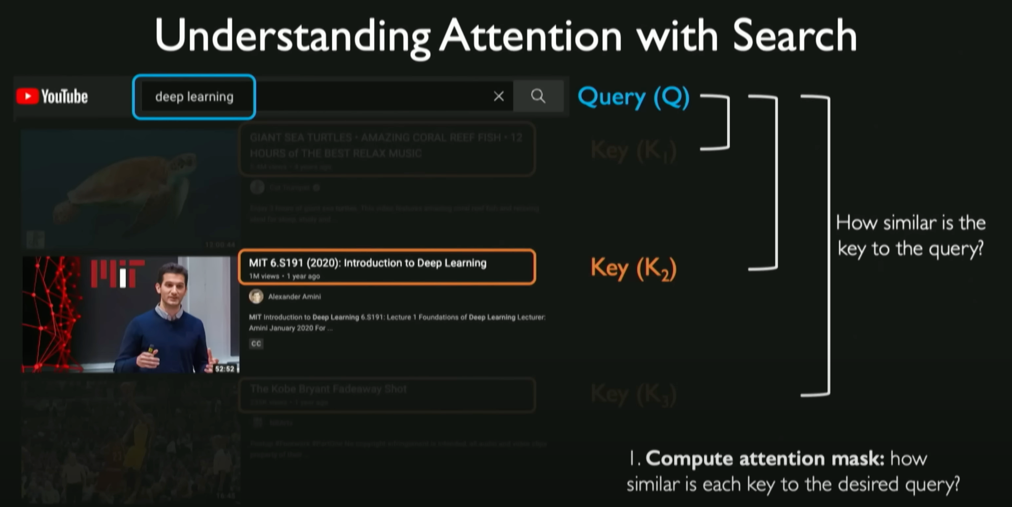
Analogy of Search Operation:
- When performing a web search, such as searching for videos on YouTube, you input a query (e.g., “deep learning”), and the search algorithm finds the videos related to that query from a vast database. This process involves identifying the similarity and relevance between each video title (as “keys”) and the query.

Similarity Calculation:
- A key operation in the search process is calculating the similarity between the query and each video title in the database. This similarity calculation helps determine which videos are most relevant to the query.
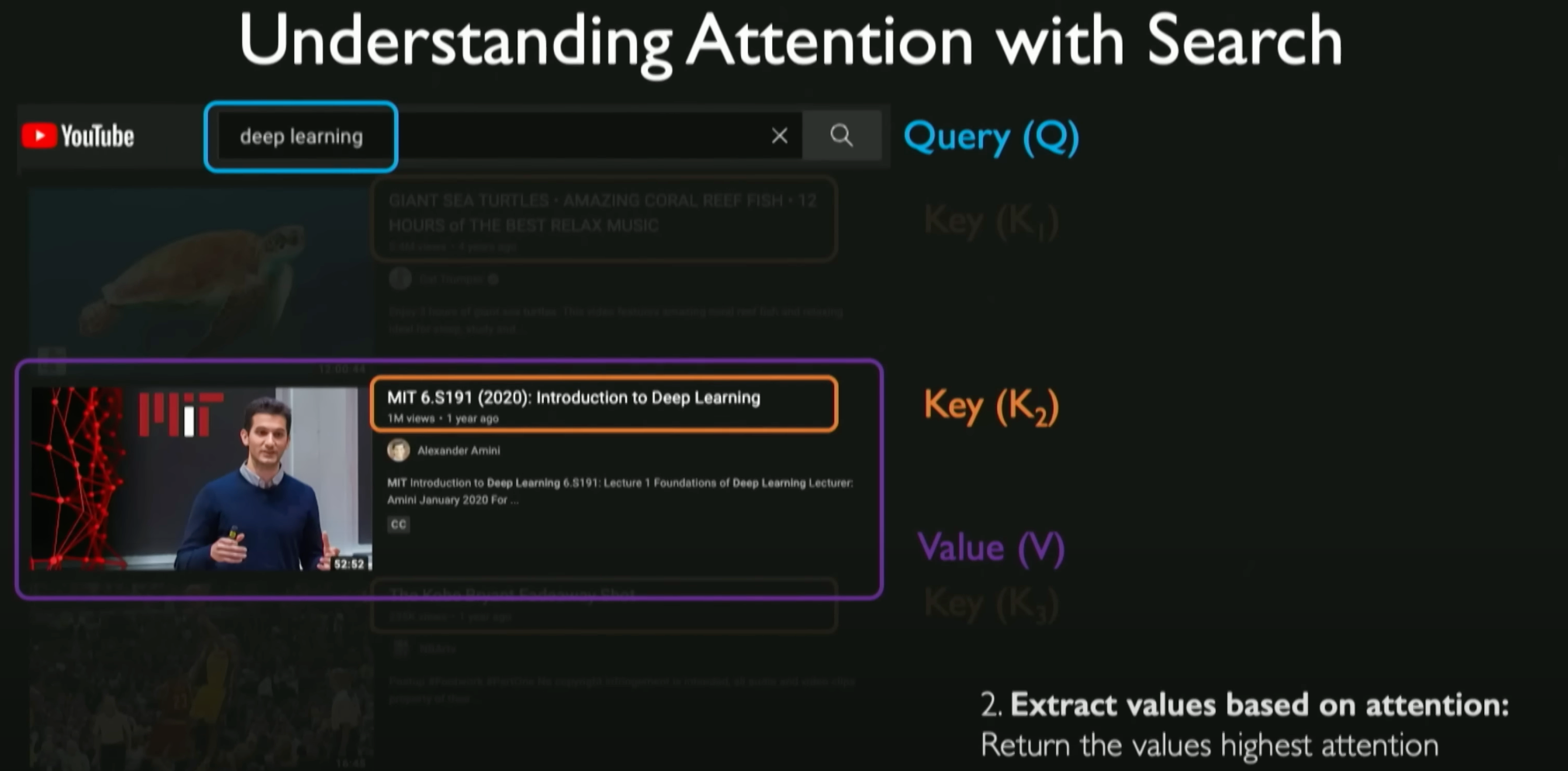
Extracting Relevant Information (Value):
- Once the most relevant videos (keys) are identified, the search operation extracts the information related to those keys, i.e., the video content (called “value”). This information extraction process is the core of Self-Attention, i.e., identifying and focusing on the information most relevant to the query.
Fundamentals of Self-Attention:
- In neural networks, especially in architectures like Transformers, the self-attention mechanism follows a similar process. The network generates query, key, and value, then calculates the similarity score between the query and the key. Based on these scores, the network extracts the values associated with high scores, representing the most important features in the input data.
Key Operations:
- The key to the self-attention mechanism is identifying which parts of the input data are most important and extracting relevant information. This mechanism allows the network to handle and understand complex sequential data effectively without relying on step-by-step recurrent processing.
Learning Attention with Neural Networks
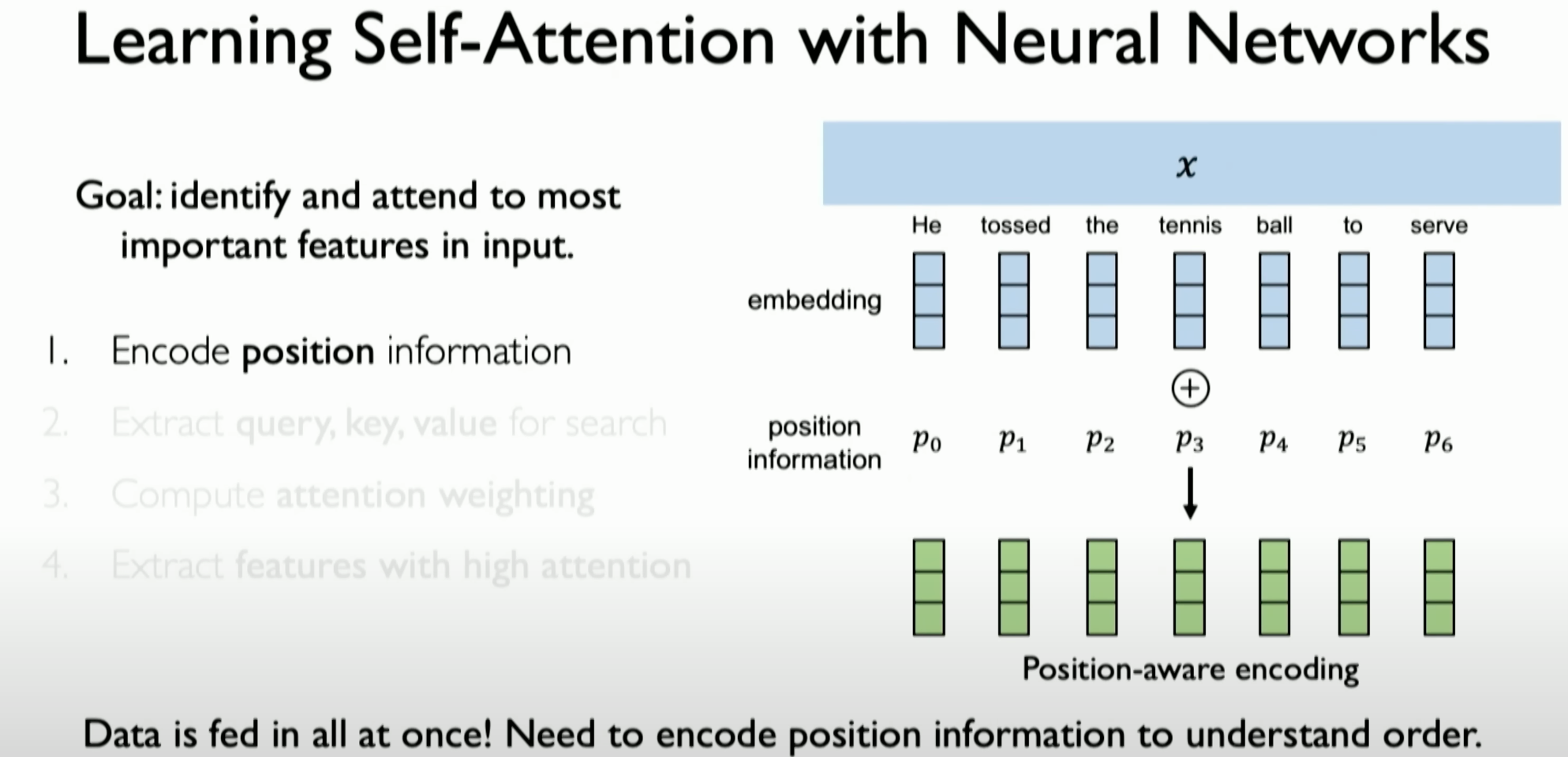
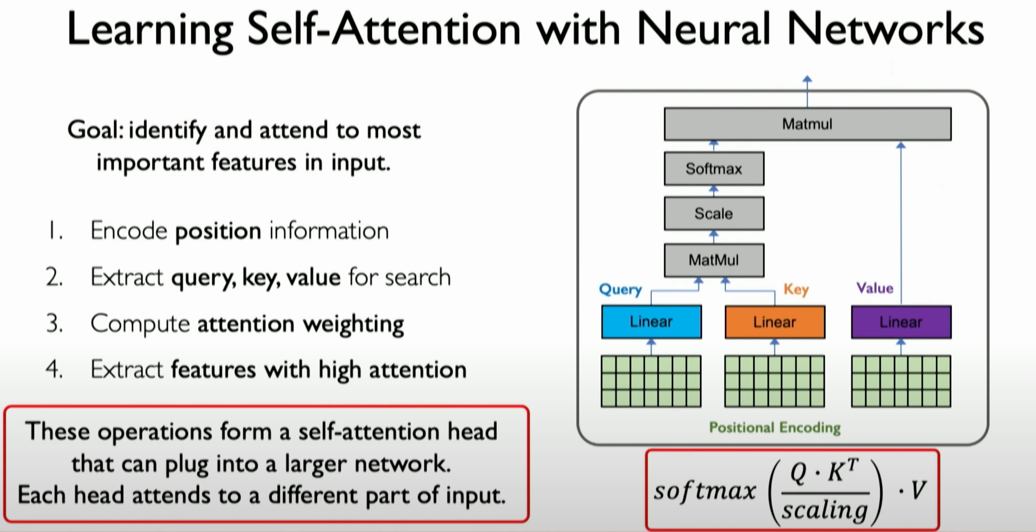
Positional Encoding:
- To handle sequential data, the first step is capturing the order information of elements in the sequence through positional encoding. Similar to the previously mentioned concept of embedding, this encoding transforms order information into a form that neural networks can process.
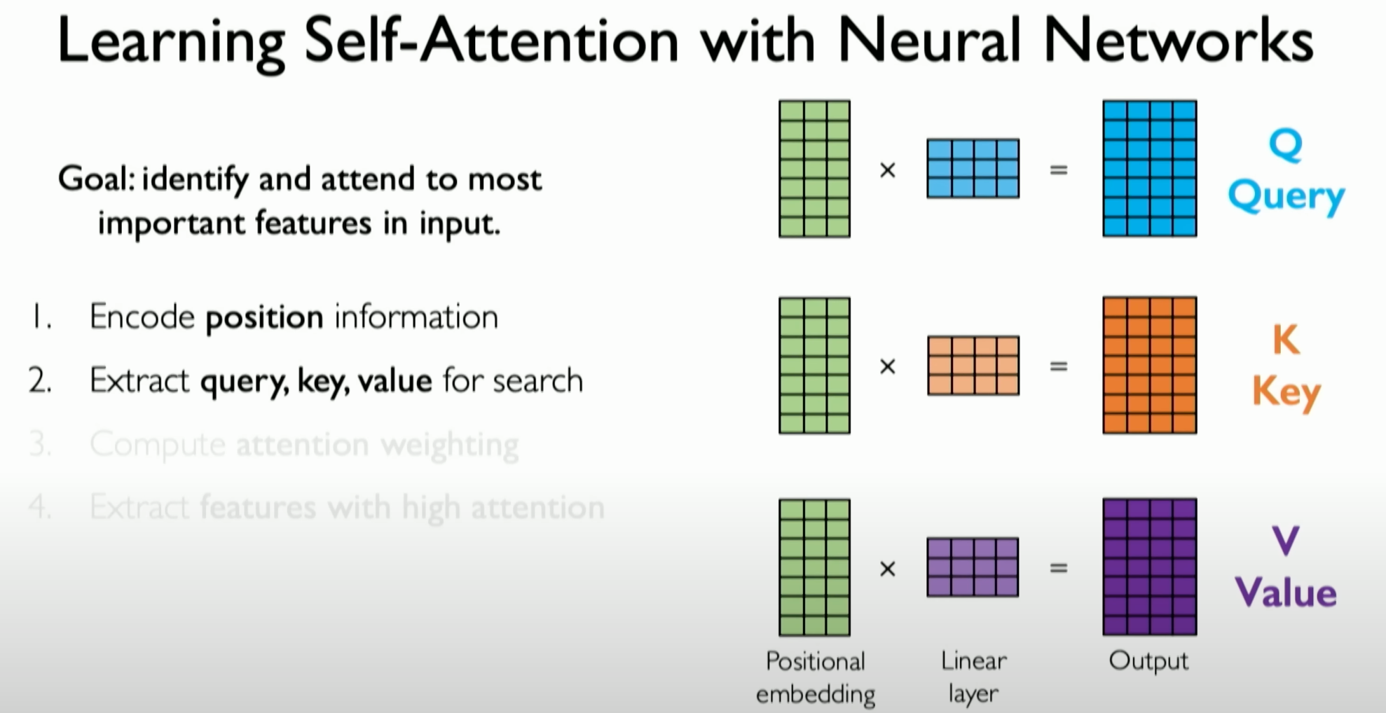
Extraction of Queries, Keys, and Values:
- Using neural network layers to process data with positional encoding, generating queries, keys, and values. These components are the core of the attention mechanism, used to determine which parts of the input data the network should focus on.
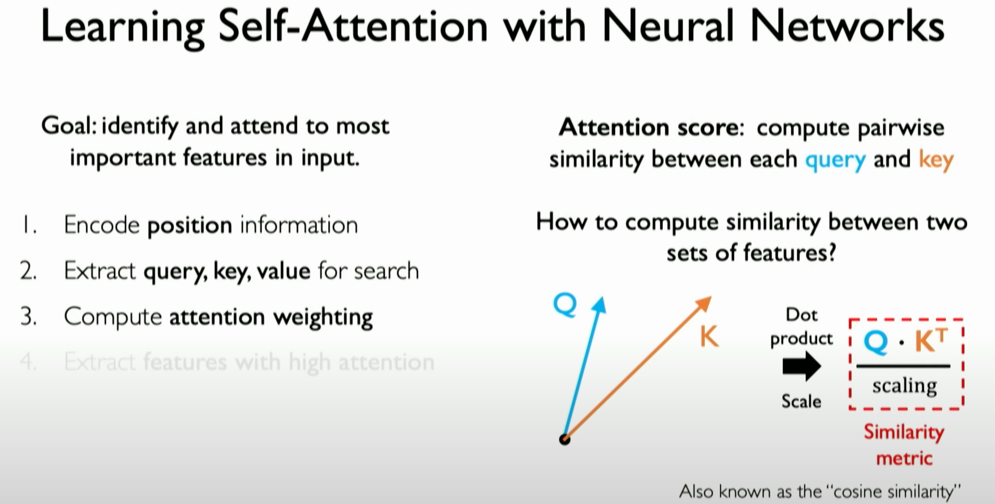
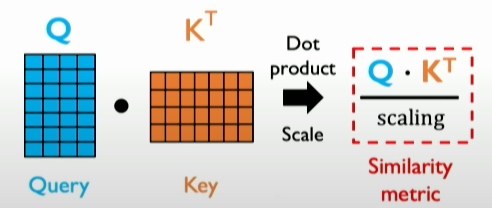
Similarity Measure:
- Calculating similarity scores between queries and keys, representing the relative importance of different parts of the input data. Typically, this similarity is achieved by computing the dot product between the query and key vectors and then scaling it.
Attention Weight Calculation:
- Converting the similarity scores through a Softmax function to obtain attention weights. These weights reflect the relative importance of different parts of the sequence.
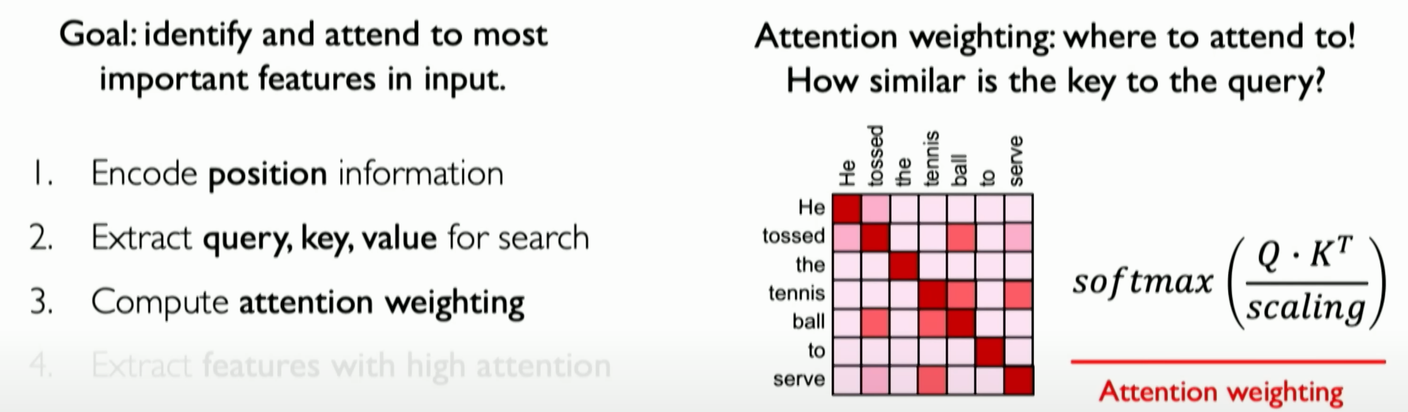
This matrix indicator itself is our attention (attention weighting), and we use the Softmax function to limit these values between 0 and 1.
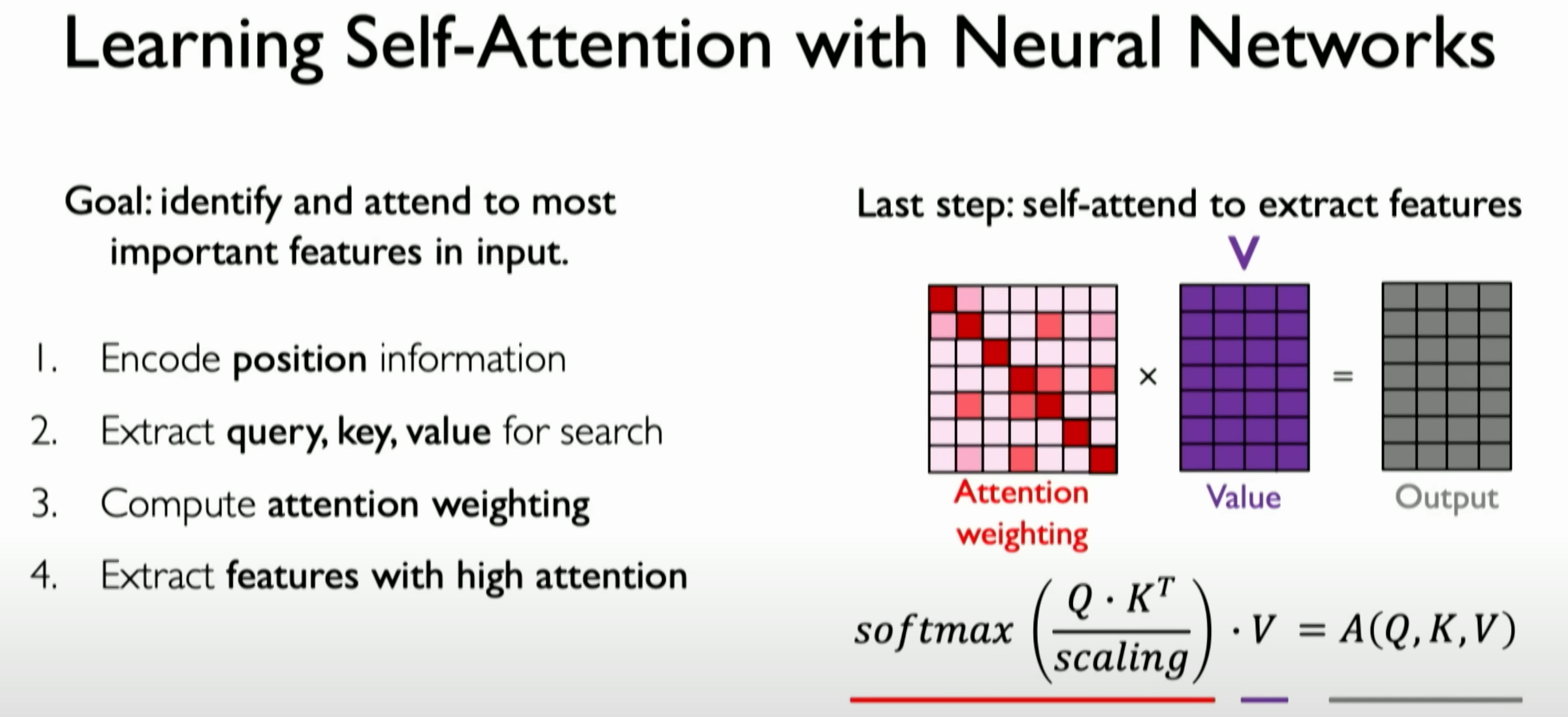
Feature Extraction:
- The final step is generating the transformed output using the attention weight matrix and values. This output reflects the important features that the network deems should receive higher attention.
Application of Self-Attention:
- The self-attention mechanism enables the model to handle and understand complex sequential data effectively without relying on step-by-step recurrent processing. It allows various components within the network to interact and extract important features based on these interactions.
This process demonstrates how the attention mechanism enables neural networks to process sequential data more intelligently by focusing on the most important parts of the input, thereby enhancing the model’s performance and efficiency. The attention mechanism is critical in the Transformer architecture, changing how models handle sequential data and improving their ability to process long sequences and complex data.
Scaling Attention and Applications
Let’s try to build our self-attention head.
- Purpose of Self-Attention:
- The core goal of the self-attention mechanism is to eliminate the need for recurrence while being able to focus on the most important features in the input data. This is the foundation of the Transformer architecture.
- Positional Encoding:
- The first step is applying positional encoding to the input data, which helps retain the order information of elements in the sequence.
- Applying Neural Network Layers:
- By applying neural network layers, positional encoding is transformed into three key components: keys, queries, and values. These components are the foundation of the self-attention mechanism.
- Calculating Self-Attention Weight Scores:
- Calculating the similarity between queries and keys through dot product operations to obtain self-attention weight scores.
- Feature Extraction:
- Using self-attention weight scores and values to extract features that deserve high attention.
- Power of Self-Attention Heads:
- The above operations define a single self-attention head. By linking multiple such self-attention heads together, a larger network architecture can be built. Different self-attention heads can extract information from different parts of the input data, forming a rich representation of the
data.
7. Building Rich Data Representations:
- Combining these different self-attention heads allows the creation of very rich data encodings and representations, enabling a comprehensive understanding and processing of the data we are handling.
In summary, the self-attention mechanism and the Transformer architecture enable handling complex sequential data by efficiently focusing on key features in the input and combining multiple self-attention heads to extract rich and diverse information. This architecture demonstrates significant potential and effectiveness in deep learning and sequential modeling.
Let’s return to the Iron Man example:
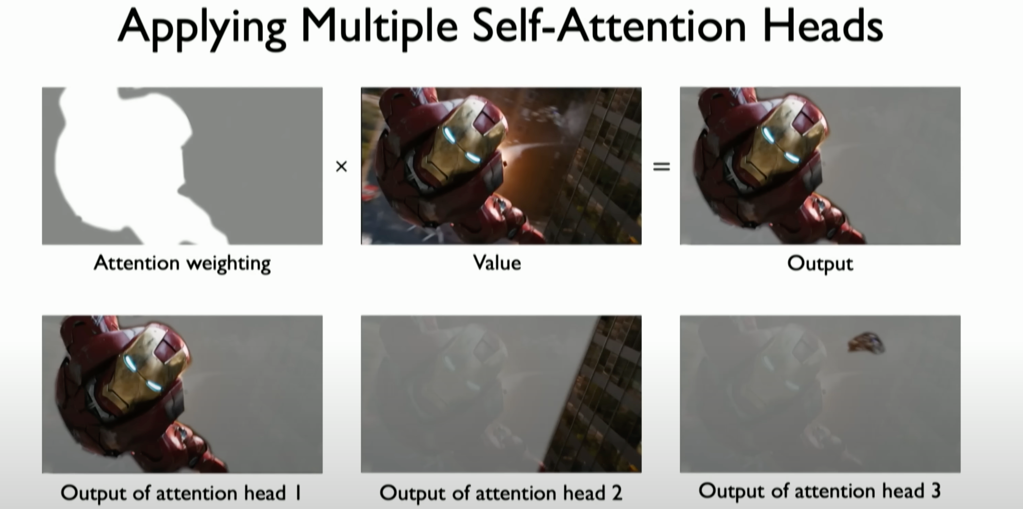
The Iron Man example shows how multiple self-attention heads extract different salient features and information from the data:
- Role of Multiple Attention Heads:
- In the Iron Man example, the first self-attention head may focus on identifying the main element of Iron Man, while other self-attention heads may identify other relevant parts that were previously unnoticed, such as the background buildings or the spaceship chasing Iron Man.
- Building Rich Data Representations:
- These different attention heads work together to select multiple relevant parts of the input data, collectively building a very rich data representation. This allows the model to understand and process the data from multiple perspectives.
- Application in Neural Network Architectures:
- The concept of multiple self-attention heads is a key building block for many powerful neural network architectures, such as the Transformer model. These architectures use different self-attention heads to extract and process various information, forming a comprehensive understanding of the data.
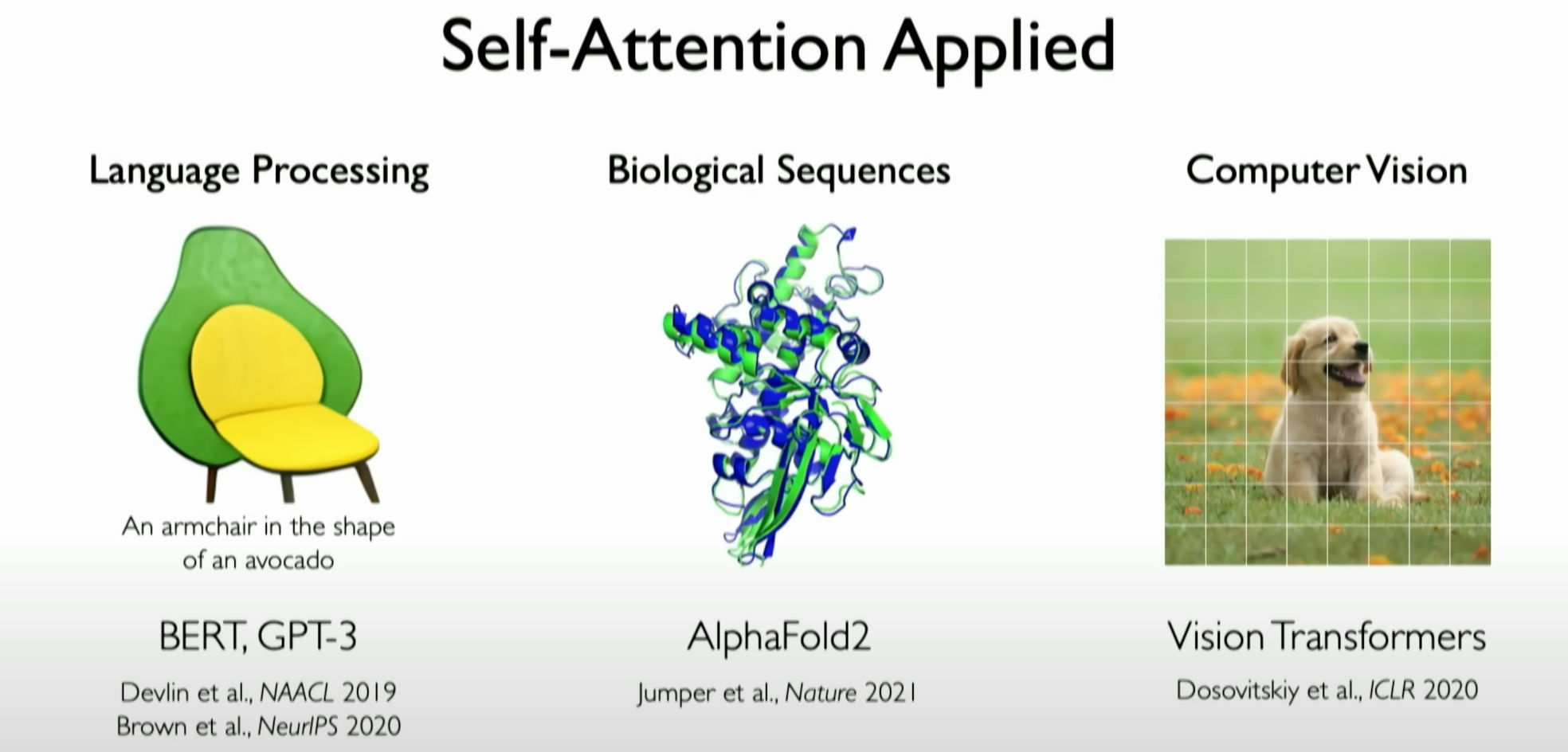
- Wide Application Range:
- The self-attention mechanism is applied not only in language models (e.g., GPT-3) to synthesize human-like natural language but also in biology and medicine (e.g., AlphaFold 2) to predict protein structures, and even extends to the field of computer vision.
Summary
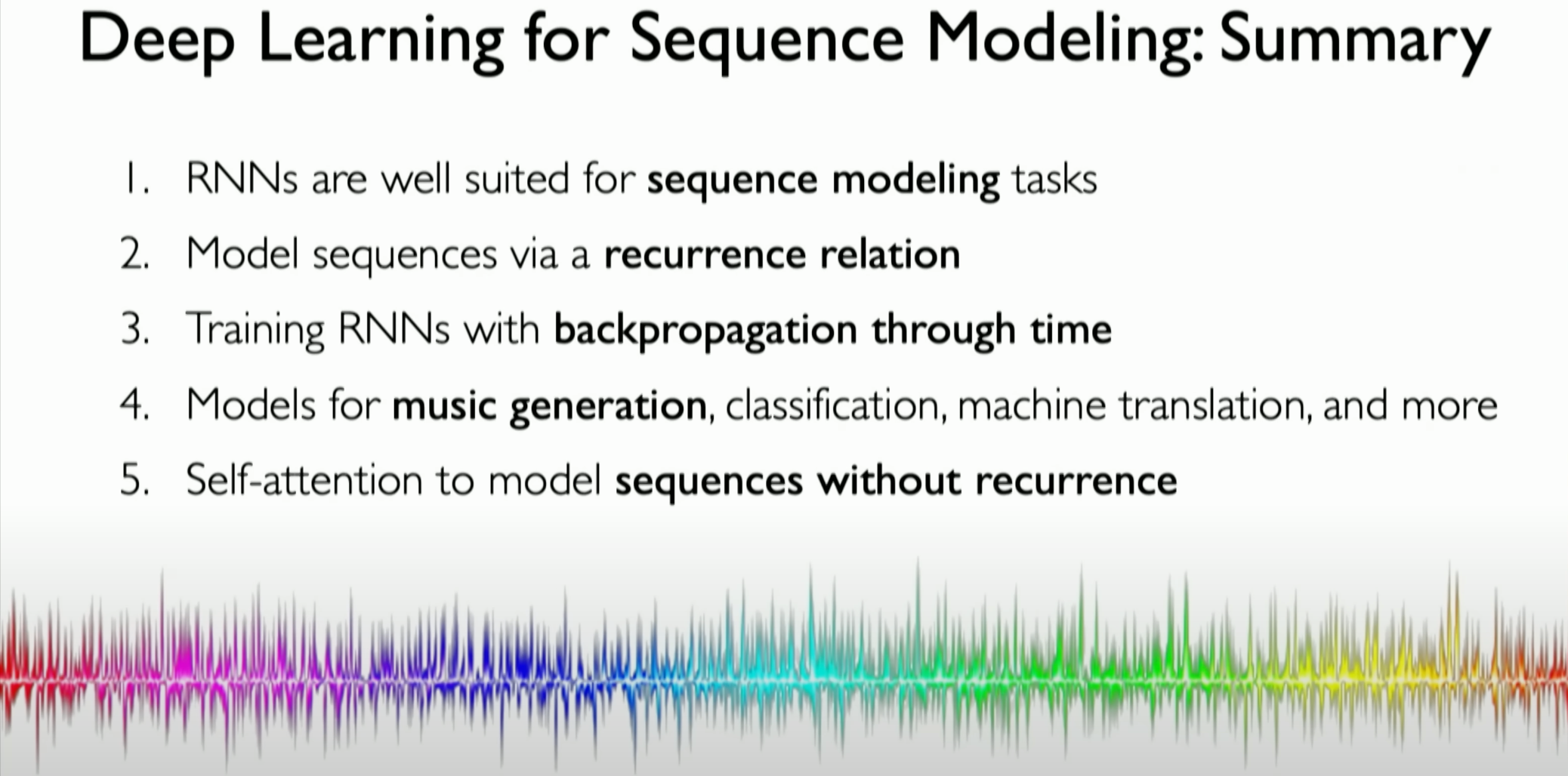
Here is a summary of the application of deep learning in sequence modeling:
RNNs are well-suited for sequence modeling tasks:
Recurrent Neural Networks (RNNs) are very suitable for sequence modeling tasks.Model sequences via a recurrence relation:
Model sequences through a recurrence relation.Training RNNs with backpropagation through time:
Train RNNs using the backpropagation through time algorithm (BPTT).Models for music generation, classification, machine translation, and more:
Models for music generation, classification, machine translation, and more.Self-attention to model sequences without recurrence:
Use self-attention mechanisms to model sequences without the need for recurrent processing.
RNNs hold a significant position in sequence data modeling by maintaining the temporal relationship of data through recurrent processing and training with the backpropagation through time algorithm. The self-attention mechanism models sequential data without recurrent processing, providing a more efficient method. These techniques have been applied to music generation, text classification, machine translation, and various other fields.
CN
Introduction
本部分专注于 sequence modeling(序列建模)的概念,以及如何构建能够处理和学习序列数据的神经网络。讲座开始时,介绍了序列建模在理解和处理涉及序列处理的数据(如语言、音频、金融市场和生物序列)中的重要性。
强调了理解神经网络功能基础并在序列建模背景下发展 intuition(直觉)的重要性。介绍了 recurrence(递归)的概念,并解释了 Recurrent Neural Networks-循环神经网络(RNN)是如何设计来处理序列数据的。这包括了解网络的 internal state(内部状态)或 memory(记忆),以及随着新数据的处理,它是如何随时间更新的。
物体的轨迹
声波
语言
通过实际例子来阐明序列数据在日常环境中的存在,例如在移动物体的轨迹、声波和语言中。这些例子强调了序列建模在现实世界应用中的相关性。接着,解释了 embedding(嵌入)的概念,这对于将文本数据转换成神经网络可以处理的数值格式至关重要。
还涵盖了RNN的关键设计标准,如处理 variable sequence lengths(可变序列长度)、tracking dependencies over time(跟踪随时间的依赖性)以及维护序列中的顺序。讨论了这些设计标准如何激发对强大架构(如Transformers)的需求,这些架构在序列建模任务中可以超越RNN的性能。
最后,讨论了训练RNN的过程,重点是 backpropagation algorithm(反向传播算法)及其对序列数据的调整,称为 backpropagation through time(时间反向传播)。这一部分突出了有效处理序列数据时训练RNN所涉及的技术细节。
Sequence modeling
sequence modeling有多种应用场景,我们按照其输入输出的可以粗略将其分为:一对一(二分类问题),多对一问题,一对多问题,多对多问题
第二部分的内容关注于序列建模,探讨了循环神经网络(RNN)、长短期记忆网络(LSTM)以及注意力机制的原理和应用。
序列建模的重要性:序列建模对于理解神经网络如何处理可变长度序列至关重要。这包括追踪不同长度序列中的依赖关系,例如在长句子中保持早期信息的相关性。
Neurons with recurrence
“具有递归性的神经元(Neurons with Recurrence)”部分的详细内容包括以下几个方面:
递归的概念与递归神经网络的定义:首先,课程介绍了递归(recurrence)的概念,这是为了构建对递归神经网络(Recurrent Neural Networks,简称RNN)的理解。递归神经网络是处理序列数据的强大工具。
从感知器到递归神经网络:课程从感知器(perceptron)的基本概念开始,解释了如何通过增加递归性来扩展神经网络的概念。感知器是单一的神经元操作,其中多个输入乘以相应的权重,并通过非线性激活函数生成输出。但在传统的感知器或前馈神经网络中,不考虑输入数据的时间顺序或序列性质。
在前馈神经网络的案例中,就算它将多个 perceptron 堆叠(stack)在一起,我们依然没有 temporal processing 或 sequential information 的概念
时间步长与内部状态的概念:引入了时间步长(time step)的概念,这是理解RNN的关键。RNN在处理数据时考虑了时间步长。这意味着网络的输出不仅取决于当前的输入数据,还取决于过去的内部状态或记忆。
我们尝试简化 inputs 和 ouputs 之间的 perceptrons 的处理过程,用一个简单的绿色块来代替,里面的处理过程并没有任何变化,现在我们新引入了一个新的变量
T,我们用它来表示单个 time step(时间步长)递归关系与内部状态的更新:RNN通过所谓的递归关系(recurrence relation)维护和更新其内部状态(internal state)。这个递归关系确定了网络在特定时间步长的计算是如何被传递到后续时间步长的。这种内部状态的更新在数学上与其他神经网络操作相似,但它同时考虑了当前输入和先前时间步长的状态。
在此处,我们定义了一个变量
H,它被称为 internal state(内部状态),它由 neurons 和 network 共同维护,它会在我们处理序列信息时同步作为 time step 进行输入,这意味着我们输入的数据不止有输入的dataX,同时也包含了一个有着捕获 memory 的概念,且会随着神经网络传递并动态改变的 internal state ——>H,RNN的计算图展开:介绍了RNN的计算图如何随时间展开,解释了每个时间步长是如何独立处理并最终累加以形成整体输出的。
Recurrent neural networks
RNN的数学定义和编码实现:详细描述了RNN的数学定义和如何在代码中实现。强调了RNN是如何通过保持状态并在每个序列处理时更新状态来工作的。
我们通过一个数学描述来理解 internal state 的更新过程,即在每一个时间步,通过以一个新的 function W,将当前 time step 的 inputs X of t,和上一个 internal state,作为输入,从而计算得到当前 time step 的 internal state。
RNN Intuition
- 循环的概念(Recurrence Concept):讲师通过与传统感知器的对比,引入了循环的概念。在感知器中,输入被视为独立的,而不是序列中的一部分。但在RNN中,输入被视为序列的一部分,网络的输出不仅取决于当前输入,还取决于先前的输入。
- 时间步和状态(Time Steps and States):RNN在处理数据时考虑时间步(time step)。讲师指出,RNN的每一步操作都是基于当前输入和之前时间步的内部状态(或称为“记忆”)。
- 状态的更新(State Update):RNN利用递归关系(recurrence relation)来维护和更新其内部状态。这种关系定义了网络在一个特定时间步的计算如何影响后续时间步的计算。
- RNN的实现(RNN Implementation):讲师介绍了RNN的实际实现方式,包括如何在Python代码中定义RNN,以及如何初始化其隐藏状态和处理输入序列。
1 | # Create an RNN instance |
上面是实现这一过程的伪代码。
Unfolding RNNs
我们可以看到RNN的计算包括:对 hidden state 的更新,以及生成一些 predicted output,那就是我们感兴趣的最终目标。
循环神经网络(RNN)的基本计算过程可以分为以下几个步骤:
输入和隐藏状态的初始化:RNN 开始时,你需要初始化输入数据和隐藏状态。输入数据通常是序列数据,比如一系列单词或时间序列数据。隐藏状态是RNN记忆先前输入的机制,一般在开始时初始化为零或一个小的随机数。
每个时间步的处理:对于序列中的每个元素(例如,一句话中的每个单词),RNN都会执行一系列计算,这些计算涉及当前输入和上一时间步的隐藏状态。
a. 输入处理:当前时间步的输入数据被处理。如果输入数据是诸如文本之类的非数值数据,它首先需要被转换成数值形式,通常是向量(例如,通过词嵌入)。
b. 隐藏层计算:RNN 通过结合当前时间步的输入和上一时间步的隐藏状态来更新其隐藏状态。这通常涉及一个或多个线性变换(加权求和)和非线性激活函数。公式通常是这样的:
,其中 是当前隐藏状态, 是前一个隐藏状态, 是当前输入, 和 是模型参数, 是激活函数,如 tanh或ReLU。c. 输出预测:
基于更新后的隐藏状态,RNN会计算当前时间步的输出。这也可能包括线性变换和激活函数。在某些应用中(如语言模型),输出可能是对序列中下一个元素的预测。公式可以是,其中 是输出。 序列处理:以上步骤对序列中的每个元素重复执行,直到处理完整个序列。
输出序列:根据应用,RNN可以输出最后一个时间步的输出,或者整个序列的输出。
误差反向传播和参数更新:在训练RNN时,你会根据输出和实际值计算误差,并通过反向传播算法更新网络的权重,以最小化这个误差。
RNN特别适合处理序列数据,因为它们能够捕捉序列中的时间动态。然而,传统的RNN有梯度消失和梯度爆炸的问题,这限制了它们在处理长序列时的有效性。为解决这一问题,已经开发了更复杂的RNN变体,如长短时记忆网络(LSTM)和门控循环单元(GRU)。
RNN的展开,可以表示为一个递归复用的网络,我们只是简单的在每一个独立的 time step 重复使用三个相同的 weight matrics,这些矩阵在每个时间步对输入数据和隐藏状态进行操作,以生成新的 hidden state 和 output。这三组权重矩阵分别是:
**输入到隐藏状态的权重矩阵
**: - 这个矩阵用于处理当前时间步的输入数据。
- 它将输入数据转换为一个与隐藏层大小相匹配的形式。
- 在每个时间步,当前的输入
与这个矩阵相乘,形成输入的一部分对隐藏状态的贡献。
**隐藏状态到隐藏状态的权重矩阵
**: - 这个矩阵用于处理前一时间步的隐藏状态。
- 它定义了如何根据前一时间步的隐藏状态
更新当前的隐藏状态。 - 这个矩阵是RNN能够“记住”序列历史信息的关键因素。
**隐藏状态到输出的权重矩阵
**: - 这个矩阵用于根据当前的隐藏状态生成输出。
- 它将隐藏状态转换为最终输出,例如,在语言模型中可能是下一个单词的概率分布。
- 这个矩阵决定了当前隐藏状态如何影响输出结果。
在每个时间步中,RNN使用这些矩阵通过以下步骤生成输出和更新隐藏状态:
- 首先,当前输入
与 相乘。 - 同时,前一时间步的隐藏状态
与 相乘。 - 这两个结果相加,并应用一个激活函数(如
tanh或ReLU),以产生新的隐藏状态。 - 新的隐藏状态
可以用于生成输出,方法是将其与 相乘。
这种重复使用权重矩阵的机制是RNN处理序列数据的基础,允许网络通过时间传递信息,并根据过去的信息做出决策。
RNNs from scratch
训练循环神经网络(RNN)并定义损失的过程涉及以下几个关键步骤:
1. 初始化权重矩阵和隐藏状态
- 权重矩阵:初始化RNN中用于输入到隐藏状态、隐藏状态到隐藏状态以及隐藏状态到输出的权重矩阵。
- 隐藏状态:通常初始化为零。这是RNN保持过去信息的机制,它会随着每个时间步的输入而更新。
2. 前向传播
- 在每个时间步,RNN接收一个输入(
)并更新隐藏状态( )。 - 隐藏状态的更新是基于当前输入和上一个时间步的隐藏状态。
- 更新后的隐藏状态用于生成当前时间步的输出。
3. 计算损失
- 在每个时间步,RNN的输出与真实标签进行比较,计算出该时间步的损失
。 - 对于序列生成任务(如语言模型),通常使用交叉熵损失函数。
- 对于序列分类任务,损失可能仅计算在最后一个时间步的输出。
- 总损失
是所有时间步损失的累积。
4. 反向传播和权重更新
- 使用反向传播算法(如梯度下降),根据总损失更新权重矩阵。
- 在反向传播过程中,误差信号从输出层回传到输入层,通过每个时间步的隐藏状态。
5. 迭代训练
- 重复前向传播、计算损失、反向传播和权重更新,直到模型达到满意的性能。
实现示例
从零开始定义:
1 | import tensorflow as tf |
TensorFLow未来提供了抽象的API实现,我们可以非常简单的调用API来实现自己的RNN。
在TensorFlow中实现RNN时,可以定义一个RNN层类。这个类包括权重矩阵的初始化、隐藏状态的更新方法,以及如何根据隐藏状态生成输出。这个过程会在每个时间步重复进行,以处理整个输入序列。
1 | import tensorflow as tf |
在这个例子中,SimpleRNNLayer 类处理单个时间步的操作,而 SimpleRNNModel 类管理整个序列的处理。这个模型可以根据特定的任务进行训练和优化。
Design criteria for sequential modeling
在处理序列建模问题时,RNN需要满足以下四个设计标准:
处理可变长度序列:RNN模型应能够处理不同长度的序列。这意味着无论序列是短还是长,模型都应能有效处理。
追踪和学习时间相关依赖性:RNN的一个关键任务是能够追踪和学习数据中随时间发展的依赖关系。这可能包括在时间上相距很远的不同元素之间的依赖性。
保持顺序信息:序列数据的一个基本特征是当前输入依赖于先前输入的特定顺序。RNN需要能够保持这种顺序信息,因为观察到的顺序对最终的预测结果有重要影响。
参数共享:RNN需要实现参数共享,这意味着同一组权重应该能够应用于序列中的不同时间步,从而产生有意义的预测。这有助于模型在处理各种时间步的数据时保持一致性和有效性。
这些设计标准是为了确保RNN能够有效地处理序列数据,同时也是推动研究和开发更强大架构的动力,这些架构可能在序列建模方面超越RNN的性能。
Word prediction example
问题描述:给定一系列单词,任务是预测句子中的下一个单词。例如,给定句子“This morning I took my cat for a walk.”,任务是预测句子中的最后一个单词。
将语言信息转换为数值编码:在考虑如何定义RNN之前,首先需要确定如何将文本信息转换成神经网络可以处理和理解的数值编码形式。因为神经网络本身不具备直接处理语言的能力,它们只是执行数学运算的函数运算符。
嵌入(Embedding)的概念:将语言信息转换为数值编码的关键方式是使用“embedding ”。这是一种将词汇表中的每个单词映射到固定大小的数值向量的转换。一种常见的方法是通过定义词汇表中所有可能出现的单词,并为每个单词分配一个唯一的索引标签,创建一个所谓的“单热(one-hot)”嵌入向量。
神经网络学习嵌入:另一种方法是使用神经网络来学习嵌入,从而捕捉输入数据中的固有含义或语义,并使相关单词或输入在嵌入空间中更加紧密地联系在一起。
设计标准:处理这类问题时,RNN需要满足几个关键标准:能够处理不同长度的序列、跟踪序列数据中的依赖关系、处理顺序信息,并且能够应用参数共享的概念。
总的来说,这一部分深入讲解了如何使用RNN来处理和预测基于序列的文本数据,强调了嵌入技术的重要性以及在设计和训练RNN时需要考虑的关键要素。
Backpropagation through time
Backpropagation algorithm:Backpropagation algorithm 是用来训练循环神经网络(RNN)中权重的关键技术。这种算法是标准反向传播算法的扩展,用于处理序列信息。
反向传播的过程:在前馈神经网络中,反向传播算法通常是从输入开始,通过网络进行前向传递,然后将预测结果与实际结果进行比较,以计算损失。之后,损失通过网络进行反向传播以更新权重。在RNN中,这个过程需要针对序列数据进行调整。
第1阶段:激励传播- 前向传播阶段:在BPTT中,这一步涉及将整个输入序列(而不是单个输入)送入循环神经网络(RNN)。网络在每个时间步处理输入,并产生对应的输出。在这个过程中,网络保持并更新其内部状态(隐藏状态),这些状态捕获了序列中之前步骤的信息。
- 反向传播阶段:在序列的每个时间步,网络的预测结果会与实际目标进行比较,计算损失。与标准BP算法不同的是,这里损失是在序列的每个时间步上计算的,而不是单个输出。
第2阶段:权重更新- 在BPTT中,权重更新的过程与标准BP算法相似,但有一定的差异。首先,计算出的梯度不仅取决于当前时间步的误差,还取决于之前时间步的误差。这是因为RNN的当前状态是基于之前的所有状态计算的。
- 每个权重的梯度是通过将输入激励(在这种情况下,包括当前和之前的时间步的输入和隐藏状态)与响应误差相乘得到的。然后,这个梯度会被用来更新网络的权重,通常是通过乘以一个学习率(即“训练因子”)并取反。
迭代过程- 在BPTT中,这个迭代过程涉及整个序列。网络需要在序列的每个时间步上前向和反向传播,直到整个序列的输出达到满意的效果。这意味着BPTT需要处理更长的依赖关系,这在计算上是更加复杂和挑战性的。
总结来说,BPTT在概念上与标准BP算法类似,但它专为处理序列数据和RNN的特性(如状态的持续更新和时间步之间的依赖)而设计。这导致了BPTT在实现和执行时比标准BP算法更加复杂。
先通过每个单独的 time step 反向传播损失
接着在所有 time step 上执行反向传播的操作,即从当前时间
T一直到序列的开头,这就是该算法被称为 Backpropagation through time 的原因因为 data(数据)和 predictions(预测)以及产生的 errors(错误)会及时的反馈,从我们当前所在的位置一直到输入数据序列的开头。
时间展开:在RNN中,由于每个时间步的输出取决于当前输入和之前的隐藏状态,因此在计算梯度时,需要考虑整个输入序列。这就要求将RNN在时间上展开,以便能够追踪和更新每个时间步的状态和梯度。
损失计算和权重更新:在RNN中,每个时间步的损失需要被计算并累加以形成总体损失。然后,这个总体损失会被用于通过整个序列的每个时间步反向传播,以更新网络的权重。
Gradient issues
循环神经网络(RNN)会有的两个主要梯度问题:梯度爆炸(exploding gradient)和梯度消失(vanishing gradients)
梯度爆炸(exploding gradient)问题:
- 梯度爆炸是指在RNN的训练过程中,梯度的值变得非常大,以至于无法稳定地训练网络。这个问题通常发生在权重矩阵
很大的情况下,导致通过网络反向传播时,梯度急剧增加。 - 为了解决梯度爆炸问题,可以采用一种称为“梯度裁剪(gradient clipping)”的方法。这个方法通过限制梯度的大小,使其保持在一个合理的范围内,从而防止梯度值过大。
- 梯度爆炸是指在RNN的训练过程中,梯度的值变得非常大,以至于无法稳定地训练网络。这个问题通常发生在权重矩阵
梯度消失(vanishing gradients)问题:
- 梯度消失是指在RNN的训练过程中,梯度的值变得非常小,几乎接近于零,导致网络难以学习和更新权重。这个问题通常发生在权重矩阵
很小的情况下,导致通过网络反向传播时,梯度逐渐减小直至消失。 - 梯度消失问题是RNN特别需要关注的问题,因为它会导致RNN无法学习到输入序列中的长期依赖关系。
我们可以通过一个简单的案例来说明 vanishing gradients 的问题,处理短序列时,RNN的每个时间步之间的距离较短,这意味着网络需要学习和保持的依赖关系也较短。例如,考虑一个简单的序列“我很饿,所以我吃了一个苹果”。
在这种情况下,由于序列较短,当前单词(如“苹果”)与之前单词(如“吃了”)之间的关联很容易被捕捉。RNN的梯度可以有效地流动,因为它们不需要通过太多的时间步来回传播。
因此,在短序列中,vanishing gradients 问题不那么明显,网络能够有效地学习序列中的依赖关系。
当处理超长序列时,例如一段包含数百个单词的文本,RNN需要学习和保持的依赖关系跨越更长的时间步。这可能包括跨越整个段落的上下文关系。
在这种情况下,由于序列长度过长,梯度需要通过更多的时间步回传播。随着梯度反向传播过程中经过的每个时间步,它们可能会逐渐减少,特别是如果使用的是传统的激活函数(如tanh或sigmoid)。
这导致网络中较早时间步的梯度变得非常小,几乎接近于零,这意味着网络难以学习和保持序列中早期时间步的重要信息。结果就是,尽管网络可能在处理序列的近期信息时表现良好,但它无法有效地学习和记住长期的依赖关系。
- 梯度消失是指在RNN的训练过程中,梯度的值变得非常小,几乎接近于零,导致网络难以学习和更新权重。这个问题通常发生在权重矩阵
三种解决技巧
解决梯度消失问题的三种技巧可以概括如下:
更改激活函数:
在神经网络的每一层中更换激活函数,特别是使用ReLU(修正线性单元)激活函数。ReLU的优点在于,当输入大于零时,其导数为1,从而避免了在正输入区域的梯度消失问题。这有助于网络在正数据区域中保持较大的梯度,缓解梯度消失的问题。
参数初始化方法:
改进神经网络中参数的初始化方法,例如通过将权重初始化为 Identity matrices 单位矩阵。这样的初始化有助于防止权重在训练的早期阶段过快地缩小到零。合适的参数初始化可以确保网络在训练初期有更稳定的梯度流,防止梯度过早消失。
引入门控机制的RNN变体:
使用长短期记忆网络-long short term memory(LSTM)或其他具有门控(gating)机制的RNN变体。LSTM通过使用不同的门(如遗忘门、输入门和输出门)来控制信息流,能够有效地过滤和存储重要的信息。这种门控机制允许网络保持和更新一个独立的单元状态,这有助于在整个序列中维持梯度的流动,从而大大缓解了梯度消失的问题。
长短期记忆网络(LSTM, Long Short-Term Memory)是一种特殊类型的循环神经网络(RNN),专门设计用来解决传统RNN在处理长序列数据时面临的梯度消失和梯度爆炸问题。LSTM的关键特点是它的门控机制,这使得它能有效地学习长期依赖关系。以下是LSTM的主要组成部分和工作原理:
遗忘门(Forget Gate):
遗忘门负责决定哪些信息应该被从单元状态中丢弃或保留。它通过一个sigmoid层来实现,这一层会查看当前输入和前一个时间步的隐藏状态,输出0到1之间的数值。这个值接近0时意味着应该丢弃信息,接近1时则保留信息。
输入门(Input Gate):
输入门由两部分组成:一个sigmoid层和一个tanh层。sigmoid层决定哪些值将被更新,而tanh层则创建一个新的候选值向量,这些值可以被加到状态中。
单元状态(Cell State):
单元状态是LSTM的核心,它在整个链上运行,只有轻微的线性交互。它能够携带相关信息穿越很长的时间距离,从而保留长期的依赖关系。单元状态由遗忘门来更新,决定丢弃哪些旧信息并由输入门添加新的信息。
输出门(Output Gate):
输出门决定下一个 hidden state(隐藏状态)的值,隐藏状态包含关于当前时间步的输出信息。隐藏状态也被用于预测下一个时间步的输出。输出门查看当前单元状态并决定哪些信息将用作输出。
LSTM的这些门控机制共同作用,使得网络能够自动学习何时忘记旧信息以及何时引入新信息,这大大提高了模型在处理长序列数据时的性能和稳定性。LSTM因此在许多涉及长期依赖关系的任务中表现出色,如语言建模、机器翻译、语音识别等领域。
这三种方法各有优势,能够有效地解决或至少缓解梯度消失的问题,提高循环神经网络在处理长序列数据时的性能和稳定性。
RNN applications
这里主要介绍循环神经网络(RNN)的应用领域的两个具体例子,展示了RNN在不同领域的实际应用:
音乐生成:
- RNN可用于音乐生成,这里的任务是构建一个RNN来预测音乐序列中的下一个音符。这种应用可以用于生成全新的音乐序列,这些序列以前可能从未被创作过。
- 一个具体的例子是,几年前,一个团队使用基于RNN的模型来尝试生成著名作曲家舒伯特的未完成交响曲的第三乐章。舒伯特的这部交响曲仅完成了两个乐章,他在去世前未能完成第三乐章。使用RNN生成的音乐结果展示了RNN在音乐创作上的潜力。
情感分类:
- RNN还可以应用于情感分类任务,如处理文本数据(例如推文)并根据其内容为文本分配正面或负面标签。这种应用利用了RNN处理序列数据的能力,能够从文本序列中提取情感信息,并据此进行分类。
- 在这种情境中,RNN可以理解和分析文本中的情绪或情感倾向,如判断一条推文是表达积极(positive)情绪还是消极(negative)情绪。
这些应用示例表明,RNN由于其能够处理和分析序列数据的特性,非常适合于音乐生成和情感分类等领域。这些应用领域的多样性和实际效果展示了RNN在处理序列数据方面的强大能力。
Limitations of Recurrent Models
循环神经网络(RNN)及其变体,如长短期记忆网络(LSTM),虽然在处理序列数据方面非常有效,但它们也有一些局限性。以下是RNN的主要限制:
编码瓶颈(Encoding Bottleneck):
- RNN在处理序列数据时,需要将信息 step by step 输入和处理。这导致了所谓的“编码瓶颈”,即尝试将大量内容(例如一篇长文本)编码为单个输出,这可能只发生在序列的最后一个时间步(time step)。
- 在实际应用中,确保所有导致该时间步骤的信息都得到正确维护和编码是非常具有挑战性的,很多信息可能会丢失。
处理速度慢(Slow,no parallelization):
- 由于RNN按时间步(time step)处理数据,因此它们的处理速度可能相对较慢。RNN的这种逐步处理方式没有简单的方法可以并行化(parallelization),这限制了它们在处理大型数据集时的效率。
长期记忆能力有限(Not long memory):
- 尽管LSTM被设计来解决RNN在处理长期依赖关系时的梯度消失问题,但在实际中,RNN和LSTM处理长期依赖的能力仍然有限。RNN和LSTM难以有效处理包含数万或更多时间步骤的长序列数据,从而影响了它们学习和维护这些序列中的全部信息和模式的能力。
总体来说,尽管RNN和LSTM在处理序列数据方面表现出色,但它们在编码瓶颈、处理速度和长期记忆能力方面仍存在局限。这些限制促使研究者开发出新的架构和方法,例如Transformer,以更有效地处理序列数据。
Attention fundamentals
循环神经网络(RNN)的局限性我们之前已经提到,由于在每一个 time step 中 step by step 的处理,导致最终的三个致命问题,我们有必要去建立一种新的能够连续处理信息流的新架构。
超越RNN的需求
- 为了解决这些问题,研究人员寻求建立一种能够连续处理信息流的新架构,而不是逐步处理。
- 目标是创建一种可扩展的架构,同时保持数据中的顺序和时间依赖性,以及建立更强大的长期记忆能力。
Intuition of attention
注意力机制的提出旨在解决循环神经网络(RNN)在序列数据处理中的关键局限性,特别是编码瓶颈、处理速度慢和长期记忆能力有限,通过引入一种机制使模型能够有效地并行处理整个数据序列,而不是逐步处理(step by step),从而允许网络更专注于输入中的重要部分并构建更细致、丰富的序列数据理解。
注意力机制的引入
- 注意力(Attention)或自我关注(Self-Attention)机制被提出,用于识别并专注于序列数据中的重要信息。
- 这种机制允许模型在潜在的顺序信息流中识别并关注重要的元素,是现代深度学习和人工智能中一个极其强大的概念。
- 通过注意力机制,模型可以在保留顺序信息的同时,更有效地从输入数据中提取信息。
注意力机制的影响
- 注意力机制的引入标志着一种从逐步(step by step)的循环处理方式向更灵活、更强大的数据处理架构的转变。
- 它为处理复杂和长序列数据开辟了新的可能性,改变了计算机视觉和语言模型等领域的传统方法。
我们可以通过一张 Iron Man 的图片来直观的引入自注意力机制(Self-Attention),当我们看一张钢铁侠的图片时,我们并不是逐像素地(类似 step by step)分析整张图片,而是直接关注重要的部分,例如钢铁侠的面部和身体。这个过程反映了我们大脑内部可能正在进行的某种类型的计算。重点在于大脑如何识别并专注于图像中的关键部分,然后提取这些部分作为值得关注的特征。这一过程与注意力机制的原理相似,即在处理复杂数据(如图像或文本)时,模型能够自动识别并专注于最重要的信息部分,而不是每一个细节。
总之,超越RNN的逐步处理方法,引入注意力机制,开启了序列数据处理的新篇章。这种方法不仅提高了处理速度,还增强了模型在捕捉长期依赖关系方面的能力,从而使深度学习模型能够更有效地理解和表示复杂的序列数据。
Attention and search relationship
现在我们在引入了 Self-Attention 后会遇到两个问题:
- Identify which parts to attention to(类似于搜索问题(search problem))
- Extract the features with high attention
搜索操作的类比:
- 当进行网络搜索时,例如在YouTube上搜索视频,您输入一个query(如“deep learning”),然后搜索算法从庞大的数据库中找出与该query相关的视频。这个过程涉及识别每个视频标题(作为“key”)与查询之间的相似性和相关性。
相似性计算:
- 搜索过程中的一个关键操作是计算(
query)与数据库中每个视频标题(key)之间的相似性。这种相似性计算帮助确定哪些视频与查询最为相关。
- 搜索过程中的一个关键操作是计算(
提取相关信息(value):
- 一旦识别出哪些视频(key)与query最相关,搜索操作接着提取与这些key相关的信息,即视频内容(称为“value”)。这种信息提取过程是Self-Attention的核心,即识别和关注与query最相关的信息。
自注意力(Self-Attention)的基础:
- 在神经网络中,特别是在如Transformer这样的架构中,自注意力机制遵循类似的过程。网络生成query、key和value,然后计算query与key之间的相似性score。根据这些score,网络提取与高得分相关联的值,这些值代表输入数据中最重要的特征。
关键的操作:
- 自我关注机制的关键在于能够识别输入数据中哪些部分最重要,并据此提取相关信息。这种机制允许网络在不依赖逐步循环处理的情况下,有效地处理和理解复杂的序列数据。
Learning attention with neural networks
位置编码(Positional Encoding):
- 为了处理序列数据,首先要通过位置编码(Positional Encoding)来捕获序列中元素的顺序(order)信息。这和之前提到的Embedding概念类似,这种编码能够将顺序信息转化为可以被神经网络处理的形式。
查询(Query)、键(Key)和值(Value)的提取:
- 使用神经网络层来处理经过位置编码的数据,生成query、key和value。这些组件是注意力机制的核心,用于确定网络应该关注输入数据的哪些部分。
相似性度量:
- 计算查询和键之间的相似性分数,这些分数表示输入数据中不同部分的相对重要性。通常,这种相似性是通过计算查询和键向量之间的点积(dot product)并进行缩放来实现的。
注意力权重的计算:
- 将相似性分数通过Softmax函数转换,得到的是注意力权重。这些权重反映了序列中各个部分的相对重要性。
这个matric指标本身就是我们的注意力(attention waiting),我们所做的是将它通过softmac函数,实现将这些值限制在0和1之间。
特征提取:
- 最后一步是利用注意力权重矩阵和值来生成转换后的输出。这个输出反映了网络认为重要的特征,即那些应该获得更高关注的部分。
自我关注(Self-Attention)的应用:
- 自我关注机制使得模型能够在没有逐步循环处理的情况下,有效地处理并理解复杂的序列数据。它允许网络内部的各个组件相互关联,并根据这些关联提取重要特征。
这一过程展示了注意力机制如何使神经网络能够更智能地处理序列数据,通过关注输入中最重要的部分来提高模型的性能和效率。注意力机制在Transformer架构中尤为关键,它改变了模型处理序列数据的方式,提高了处理长序列和复杂数据的能力。
Scaling attention and applications
我们来尝试构建自己的自注意力头(self-attention head)
- self-attention的目的:
- self-attention 机制的核心目标是消除循环(Recurrence)的需求,同时能够关注输入数据中最重要的特征。这是Transformer架构的基础。
- 位置编码(Positional Encoding):
- 第一步是对输入数据应用位置编码(Positional Encoding),这有助于保留序列中元素的顺序信息。
- 应用神经网络层:
- 通过应用神经网络层,位置编码被转换为三个关键的部分:键(Key)、查询(Query)和值(Value)。这些部分是自我关注机制的基础。
- 计算自我关注权重分数:
- 通过点积(dot)操作计算query和key之间的相似性,从而得到 self-attention weight score。
- 特征提取:
- 使用self-attention weight score和value来提取值得高度关注的特征。
- 自我关注头的强大之处:
- 上述操作定义了单个self-attention head。通过将多个这样的self-attention head链接在一起,可以构建更大的网络架构。不同的self-attention head可以提取输入数据的不同部分的信息,从而形成对数据的丰富表示。
- 构建丰富的数据表示:
- 通过结合这些不同的self-attention head,能够形成非常丰富的数据编码和表示,从而更全面地理解和处理我们正在处理的数据。
总之,自注意力机制和Transformer架构通过高效地关注输入数据中的关键特征,并通过结合多个自注意力头来提取丰富和多样化的信息,使得处理复杂的序列数据成为可能。这种架构在深度学习和序列建模领域展示了极大的潜力和效果。
让我们回到Iron Man的案例:
Iron Man的案例展示了如何通过多个自我关注头提取数据中的不同显著特征和信息:
- 多个关注头的作用:
- 在Iron Man的例子中,第一个自注意力头可能专注于识别Iron Man这一主要元素,而其他的自注意力头可能识别出之前未被注意到的其他相关部分,比如背景中的建筑或追逐钢铁侠的宇宙飞船。
- 建立丰富的数据表示:
- 这些不同的注意力头共同工作,挑选出输入数据中的多个相关部分,共同构建出一个非常丰富的数据表示。这使得模型能够从多个角度理解和处理数据。
- 在神经网络架构中的应用:
- 多个自注意力头的概念是许多强大神经网络架构的关键构建块,如Transformer模型。这些架构利用不同的自注意力头来提取和处理不同的信息,形成对数据的全面理解。
- 广泛的应用范围:
- 自注意力机制不仅应用于语言模型(如GPT-3)以合成类似人类的自然语言,还应用于生物学和医学领域(如AlphaFold 2)以预测蛋白质的三维结构,甚至扩展到计算机视觉领域。
Summary
这里是对深度学习在序列建模中的应用的总结:
RNNs are well suited for sequence modeling tasks:
循环神经网络(RNNs)非常适合序列建模任务。Model sequences via a recurrence relation:
通过递归关系来建模序列。Training RNNs with backpropagation through time:
通过时间反向传播算法(BPTT)训练RNN。Models for music generation, classification, machine translation, and more:
用于音乐生成、分类、机器翻译等的模型。Self-attention to model sequences without recurrence:
使用自我关注机制来建模序列,无需递归处理。
RNNs在序列数据建模方面具有非常重要的地位,它通过递归处理来维持数据的时序关系,以及如何通过时间反向传播算法进行训练。自我关注机制在建模序列数据时不需要递归处理,这是一种更高效的方法。这些技术已经被应用于音乐生成、文本分类、机器翻译等多个领域。