Convolutional Neural Networks

EN

Introduction

The core of the Introduction section is to demonstrate the application of deep learning in computer vision, especially how deep learning enables computers to achieve “vision.” Here is a step-by-step summary based on the content of this section:

1. Course Introduction and Motivation: The course begins by emphasizing the importance of vision as one of the most crucial human senses, highlighting how people rely heavily on vision to navigate and understand the surrounding world in daily life. This part aims to spark interest and explain the potential and value of deep learning in mimicking this essential human ability.

2. Goals of the Vision System: The introduction emphasizes that the ultimate goal of building a computer vision system is not just to recognize the location of objects (“what is where”) but more importantly to understand the deeper meaning of the scene, including the dynamics of objects and predicting possible events in the scene. This capability enables computers to understand visual information more profoundly, surpassing surface recognition.

   

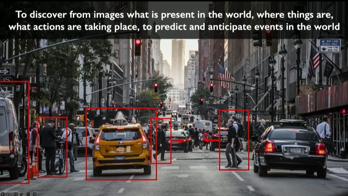
   For example, the dynamic changes of traffic lights, the walking direction of pedestrians, and more intricate details in the image above.

3. Role of Deep Learning: Through deep learning and machine learning, we can build systems capable of “seeing” and “understanding” their visual inputs. Deep learning algorithms can learn directly from raw image data without manually programming specific rules, allowing the algorithms to automatically recognize and learn complex patterns and features in images.

4. Examples of Computer Vision Applications: The introduction mentions various examples of computer vision applications, including autonomous driving, medical diagnosis, and enhancing accessibility technologies. These examples showcase the wide applications of deep learning in the field of vision and how it drives technological innovation and improves people’s lives.

5. Challenges in Deep Learning and Computer Vision: Despite significant advancements, the introduction also addresses existing challenges, such as handling high-dimensional image data, understanding spatial relationships in images, and enabling models to handle various visual variations (e.g., changes in lighting, object movement, and occlusion).

In summary, this introduction emphasizes the importance and challenges of computer vision and introduces how deep learning allows computers not only to “see” objects but also to deeply understand the complexity of visual scenes. By showcasing the potential of deep learning in various applications, the introduction inspires learners to explore how to build advanced vision systems using deep learning techniques.

Amazing applications of vision

The application of deep learning in the field of computer vision is elaborated upon, particularly its role in enabling computers to gain visual capabilities.

1. Deep Learning Leading a Revolution: Deep learning, especially over the past decade, has become the leading force in the revolution of computer vision. This technology has not only enhanced the understanding and processing capabilities of machines for images but has also extended to everyday devices such as smartphones, which can now process and enhance every captured image, including features like face detection.

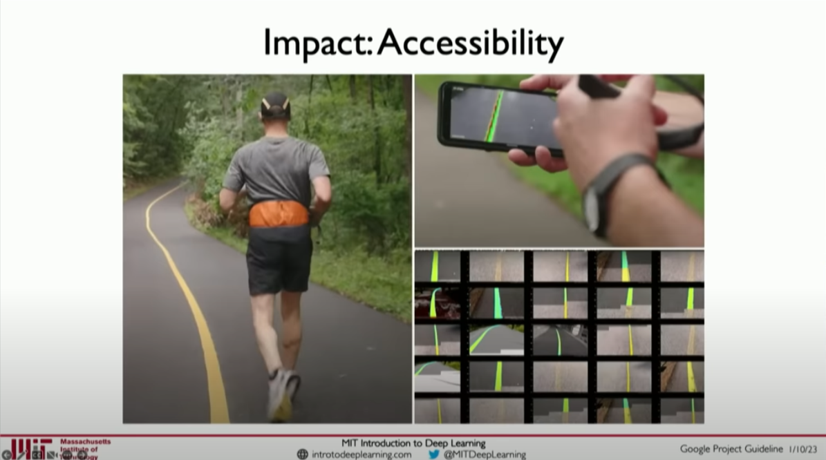
2. Application Examples: Deep learning technology has broad applications across various fields, from medicine and biology to autonomous vehicles and improving accessibility facilities. For example, deep learning is used in medical decision-making and projects that help visually impaired people navigate through sound feedback.

   

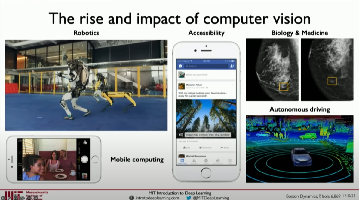
   The following is an example of predicting the trajectory and providing voice prompts to assist visually impaired runners.

   

3. End-to-End Learning Models: One major advantage of deep learning is its ability to learn directly from raw data. This means that compared to traditional methods, deep learning models can directly learn and extract features from images without manual intervention. This is particularly important in feature extraction tasks such as face detection and recognition.

   

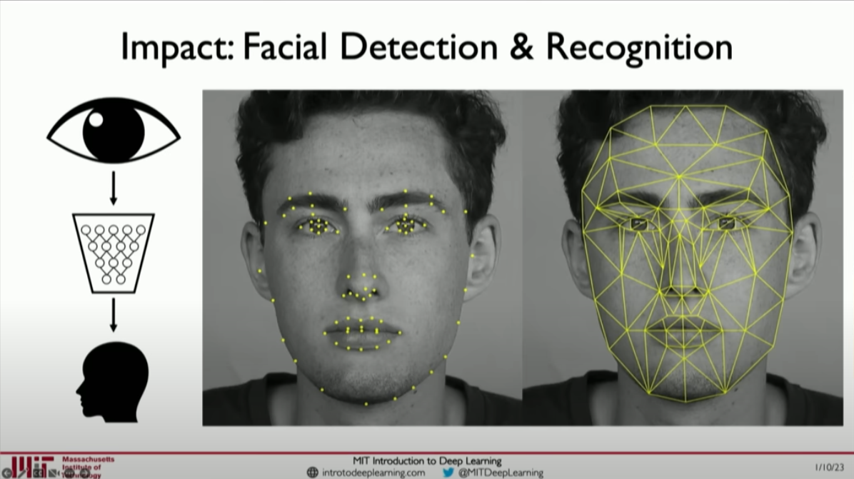
   This will also be practiced in the subsequent experiments.

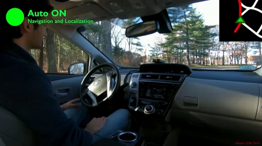
4. Example of Autonomous Driving: Autonomous driving is a significant example of computer vision applications. Deep learning models can process image or video inputs to train cars to understand their surroundings and make control decisions such as steering, accelerating, or braking. This end-to-end approach is different from the methods used by most autonomous car companies, showcasing deep learning’s potential in handling complex environments.

   

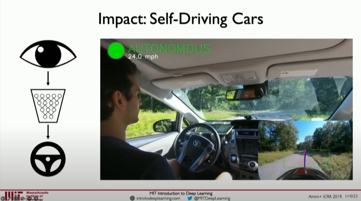
5. MIT Research Project: The text mentions an autonomous driving project developed by MIT laboratories, which demonstrates the great potential of deep learning technology in practical applications. By learning and predicting start commands, the project shows how deep learning can be applied to complex control systems.

In summary, the second section describes in detail the critical role of deep learning, especially convolutional neural networks, in advancing computer vision. From improving the image processing capabilities of smart devices to advancing autonomous driving and medical diagnosis, deep learning is opening up new applications for computer vision and showing great potential for improving human lives.

What computers “see”

Fundamentals of Computer Vision

In the field of deep learning, computer vision aims to mimic the functionality of the human visual system, enabling computers to recognize and process visual information from images or videos. A fundamental example is when we see a photo of Abraham Lincoln, we can easily identify the person. For computers, this photo is a digital matrix composed of numerous pixels, with each pixel represented by one or more values indicating its brightness and color.

Digitization of Image Data

• Grayscale Images: Each pixel is represented by a number reflecting its brightness or grayscale level.

  

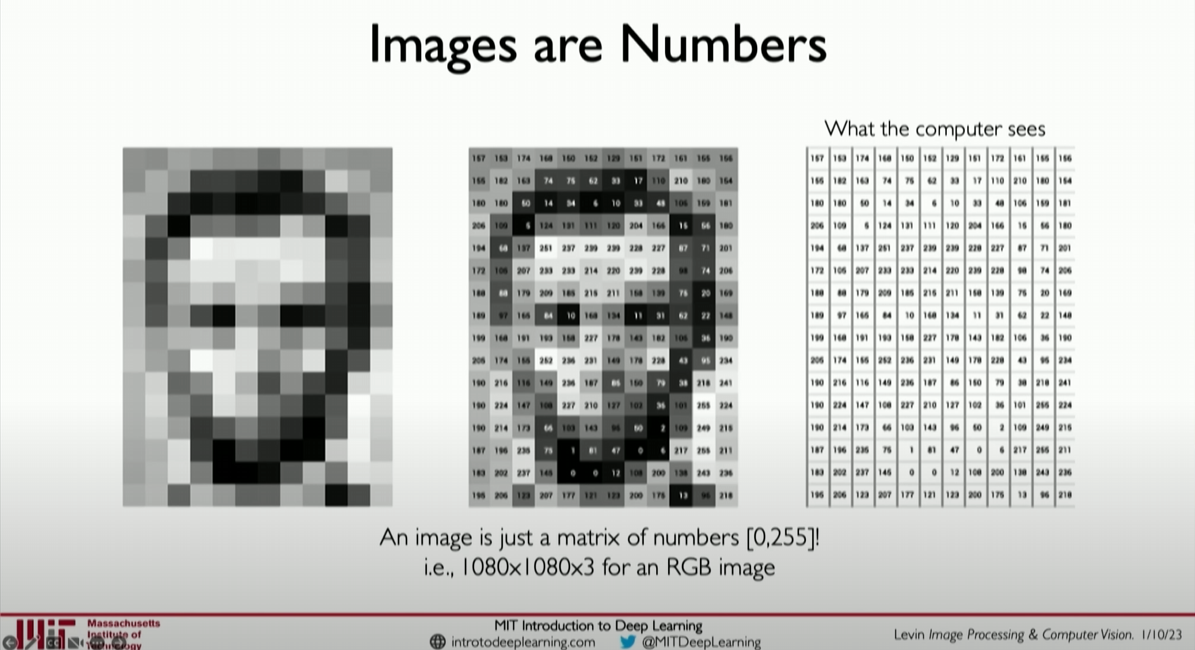
• Color Images: Typically use the RGB color model, with each pixel represented by three numbers indicating the intensity of red, green, and blue.

# Simple Python code snippet demonstrating how to represent a 2x2 grayscale image with numbers
gray_image = [[255, 0],
              [128, 128]]

# For a 2x2 RGB color image
color_image = [[[255, 0, 0], [0, 255, 0]],
               [[0, 0, 255], [255, 255, 0]]]

Image Processing Tasks

The core tasks of image processing can be divided into two categories: Classification and Regression.

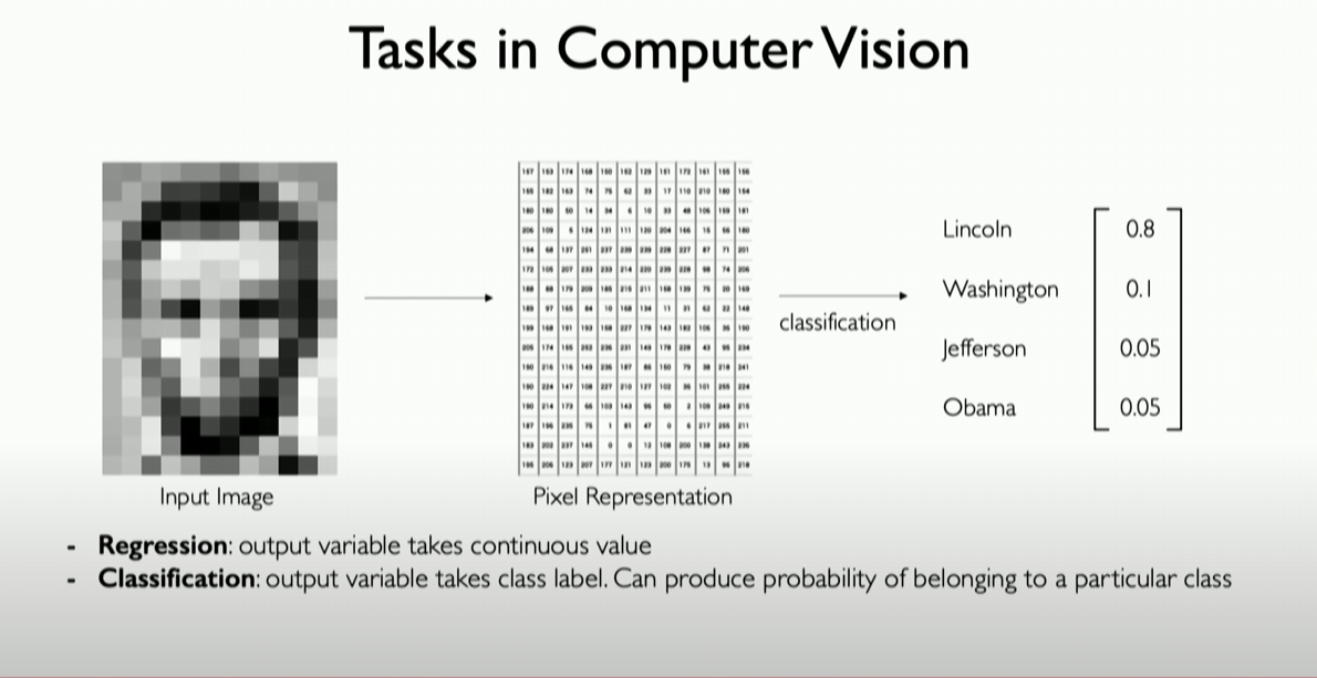
• Classification: Identifying which predefined category an image belongs to. For example, recognizing which president is in a group of presidential photos.
• Regression: Predicting continuous numerical attributes related to the image. For example, estimating the size or position of an object in an image.

Importance of Feature Extraction

First, we need to know what features or patterns to look for, and second, we need to infer which class we are currently in after detecting these patterns.

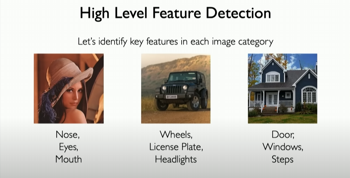
Early computer vision methods relied on manually designed feature extractors to identify patterns in images. However, these methods often struggled to accommodate the diversity and complexity of images. For example, if we want to recognize cars from photos taken at different angles, manually designed feature extractors might find it challenging to cover all possible variations.

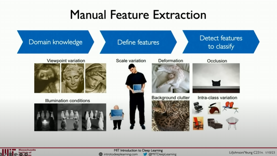
Images are essentially three-dimensional arrays of numbers, and even objects of the same category can vary greatly due to factors like occlusion, lighting changes, rotation, and translation. This makes it necessary for the classification pipeline to handle and remain invariant to these changes while remaining sensitive to differences between categories.

Even if we can manually define some features based on prior knowledge, these features often become unstable in the face of significant variations in real-world images. This raises the question of how to build a computer vision algorithm that can handle these variations while maintaining high robustness.

Solution: Utilize neural networks. Neural networks can directly learn features from data, and importantly, they can build more complex feature sets layer by layer from previously learned features. This way, from the most basic pixel-level features to semantically meaningful features (such as eyes and noses of a face), neural networks can automatically extract and recognize them in a hierarchical manner.

The Deep Learning Revolution

Deep learning introduces the concept of automatically learning features from data, achieved through the use of neural networks. A typical neural network consists of multiple layers, each capable of learning simple features (like edges and corners) and then building on those features to learn more complex features (like faces or objects).

Convolutional Neural Networks (CNN)

CNNs are a special class of networks used in deep learning for image processing. They extract features from images through convolutional layers.

# A simple CNN example (built with Keras)
from keras.models import Sequential
from keras.layers import Conv2D

model = Sequential()
# Add a convolutional layer, assuming input image size is 28x28 grayscale image
model.add(Conv2D(filters=32, kernel_size=(3, 3), activation='relu', input_shape=(28, 28, 1)))
``

`

### Hierarchical Feature Learning

CNNs can hierarchically learn features through their deep structures, allowing the model to recognize and process complex patterns in images. This hierarchical learning approach is key to CNNs' success in tasks like image classification and object detection.

In summary, deep learning, especially CNNs, has significantly advanced the field of computer vision. By automatically learning features from image data, deep learning models can process and understand various visual information from simple to complex, providing powerful support for fields such as autonomous driving and medical image analysis.

## Learning visual features

### Deep Learning and Visual Features

Deep learning, particularly convolutional neural networks (CNNs), has become the cornerstone of image recognition and processing. This is due to their ability to automatically learn complex visual features directly from raw image data without the need for manually coded feature extractors. Crucially, CNNs maintain the spatial hierarchy of images, which is vital for understanding image content.

### Problems with Fully Connected Layers

Fully connected networks (also known as dense networks) face major issues when applied to image processing tasks:

**Loss of Spatial Information**: They cannot effectively handle the spatial structure of image data. Fully connected layers flatten the image into a one-dimensional vector, causing the loss of spatial information. For instance, a fully connected network finds it challenging to distinguish different pixel patterns based on arrangement, which is unacceptable in image recognition.

**Explosive Number of Parameters**: Fully connected layers require handling a massive number of parameters, especially for high-dimensional image data. For example, a 100x100 pixel image could result in millions of parameters, making model training inefficient and unmanageable.

![image-20240408092116626](https://cdn.jsdelivr.net/gh/xiwuqi/image-hosting@master/picgo/202404080921713.png)

### Convolutional Neural Networks (CNNs)

To overcome the limitations of fully connected networks, we need a method that preserves the spatial structure of images. This means the network design should understand and leverage the spatial relationships between pixels in images.

**Local Connections and Weight Sharing**: By connecting small patches (called "receptive fields") of the input image to neurons in the hidden layer, each neuron focuses on a small part of the image. This method reduces the number of model parameters and allows the network to learn local patterns in images.

![image-20240408092232931](https://cdn.jsdelivr.net/gh/xiwuqi/image-hosting@master/picgo/202404080922987.png)

Convolutional layers solve this problem by preserving the spatial structure of images. They do this by sliding a small window (called a filter or kernel) over the image and applying the same operation at each position. This approach reduces the number of model parameters (through **weight sharing**) and enables the network to detect local patterns like edges, textures, and shapes.

![image-20240408092858431](https://cdn.jsdelivr.net/gh/xiwuqi/image-hosting@master/picgo/202404080928498.png)

#### Code Example

Here is a simple CNN architecture using Python and the Keras framework for an image classification task:

```python
from keras.models import Sequential
from keras.layers import Conv2D, MaxPooling2D, Flatten, Dense

model = Sequential([
    # First convolutional layer with 32 3x3 filters and ReLU activation function
    Conv2D(32, (3, 3), activation='relu', input_shape=(64, 64, 3)),
    # First pooling layer with a 2x2 pooling window
    MaxPooling2D(pool_size=(2, 2)),
    # Second convolutional layer with more filters to extract more complex features
    Conv2D(64, (3, 3), activation='relu'),
    MaxPooling2D(pool_size=(2, 2)),
    # Flatten layer to convert 2D convolutional output into 1D for fully connected layers
    Flatten(),
    # Fully connected layer
    Dense(128, activation='relu'),
    # Output layer with softmax activation function for multi-class classification
    Dense(10, activation='softmax')
])

model.compile(optimizer='adam', loss='categorical_crossentropy', metrics=['accuracy'])

This model is designed to process 64x64 pixel color images (3 color channels). It first extracts image features through two convolutional layers and pooling layers, then uses fully connected layers to classify these features. This structure allows the network to learn visual features from simple to complex, suitable for various image recognition tasks.

Hierarchical Feature Learning

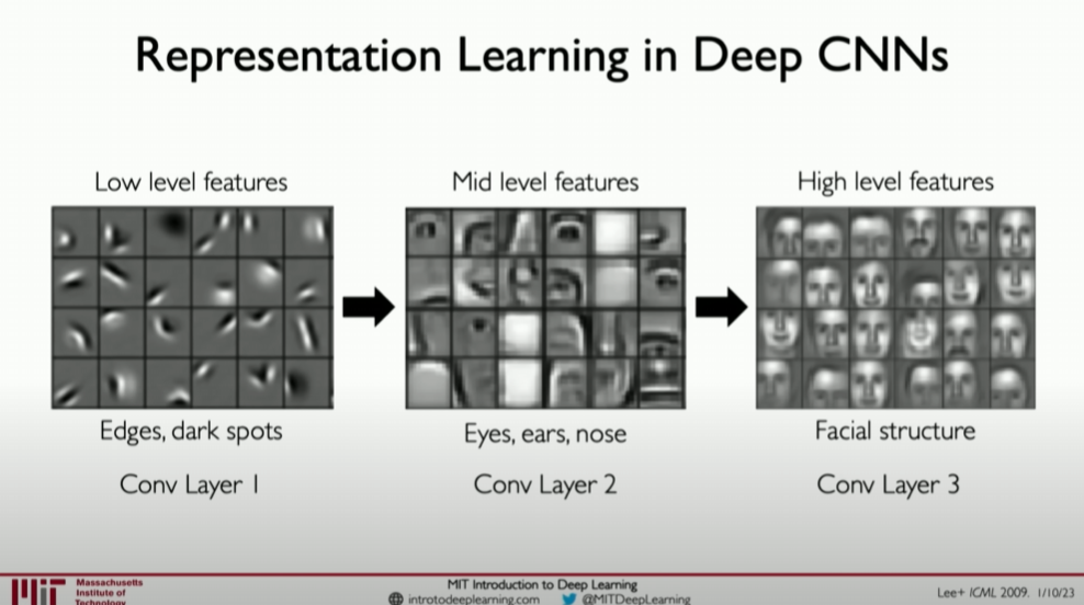
One key advantage of CNNs is their ability to hierarchically learn features. In the early stages of the network, the model learns to recognize simple visual patterns (like edges and corners). In deeper layers, the network can combine these basic features to recognize more complex structures (like parts of objects). Eventually, the model can identify high-level concepts (like specific objects or scenes).

This step-by-step learning process from raw pixels to complex concepts is key to CNNs’ remarkable success in image processing tasks. By automatically learning visual features from large amounts of labeled data, deep learning models can accurately recognize and classify images in various complex environments.

Feature extraction and convolution

To delve into the core role of feature extraction and convolution in image processing, we need to understand how convolutional neural networks (CNNs) use the convolution operation to automatically learn features from images, enabling tasks such as image classification and recognition. Convolution operations use filters (also known as convolution kernels) to identify local features in images, which can then be combined into more complex image representations.

Detailed Explanation of the Convolution Operation

Convolution is a mathematical operation that involves sliding a small window (filter) over an input image. At each filter position, the dot product between the filter and the image region it covers is computed, and the results are summed to generate a pixel value in the output image (feature map). This process is repeated until the filter covers all positions in the input image.

Role of Filters

Filters are parameters learned in convolutional networks. During training, the network adjusts the filter values using the backpropagation algorithm to better capture features in the input image. Initially, filters might detect simple edges or color changes. As layers increase, subsequent layers can combine earlier features to detect more complex patterns.

Filters determine the type of features the network can detect. For instance, some filters may specialize in detecting edges in images, while others may detect more complex patterns like diagonals or intersections.

Filters as Feature Detectors: In convolutional neural networks, each filter acts as a feature detector, looking for specific patterns in the input image. By combining the outputs of multiple such feature detectors, the network can understand and recognize complex objects in images.

Spatial Invariance

A key advantage of convolutional networks is their invariance to spatial changes in features within images. Even if objects move or rotate within the image, the features extracted through the convolution operation can still be recognized by the network. This is because filters detect features regardless of their position in the image.

Practical Example: Detecting an “X” in Images

Suppose we want to design a convolutional neural network to recognize the presence of the letter “X” in images. The letter “X” can be characterized by two intersecting diagonals. We can train the network to recognize these diagonals regardless of their position in the image.

Example Steps:

1. Initialize Filters: Initially, we randomly initialize the filter weights.
2. Slide the Filter: Slide each filter over the entire image, computing the dot product between the filter and the local image region at each position.
3. Generate Feature Maps: Calculate results at each filter position to form a new image (feature map), indicating where specific features are present in the input image.
4. Train the Network: Train the network on training data, adjusting the filters so they can better recognize the features of the letter “X,” such as diagonals and intersections.

Code Example:

Using Python and TensorFlow to build a simple CNN for recognizing images containing the letter “X”:

import tensorflow as tf
from tensorflow.keras import layers, models

model = models.Sequential([
    # Convolutional layer for detecting local features in the image
    layers.Conv2D(32, (3, 3), activation='relu', input_shape=(28, 28, 1)),
    # Pooling layer to reduce the spatial dimension of feature maps, retaining the most important features
    layers.MaxPooling2D((2, 2)),
    # Flatten layer to convert 2D feature maps into 1D vectors for fully connected layers
    layers.Flatten(),
    # Fully connected layer to further process features
    layers.Dense(64, activation='relu'),
    # Output layer for the classifier
    layers.Dense(2, activation='softmax')
])

model.compile(optimizer='adam',
              loss='sparse_categorical_crossentropy',
              metrics=['accuracy'])

# Model summary
model.summary()

In this example, the convolutional layer uses 32 filters of size 3x3 to detect small local features in the image. The pooling layer reduces the spatial dimension of these features, and the fully connected layer processes these local features into a higher-level representation for the final classification.

Conclusion

By using convolutional neural networks for feature extraction and convolution operations, we can effectively learn useful representations from images, providing powerful tools for image recognition and classification. Through training, the network can automatically learn the optimal filters needed to recognize various image patterns, achieving high accuracy in complex image recognition tasks.

The convolution operation

To understand the convolution operation and its application in automatically learning image features, we need to start with the basic working principles of convolutional neural networks (CNNs). CNNs extract useful features from input images through a series of convolutional layers, which are then used to perform various visual tasks

such as classification, detection, and segmentation.

How Convolutional Layers Work

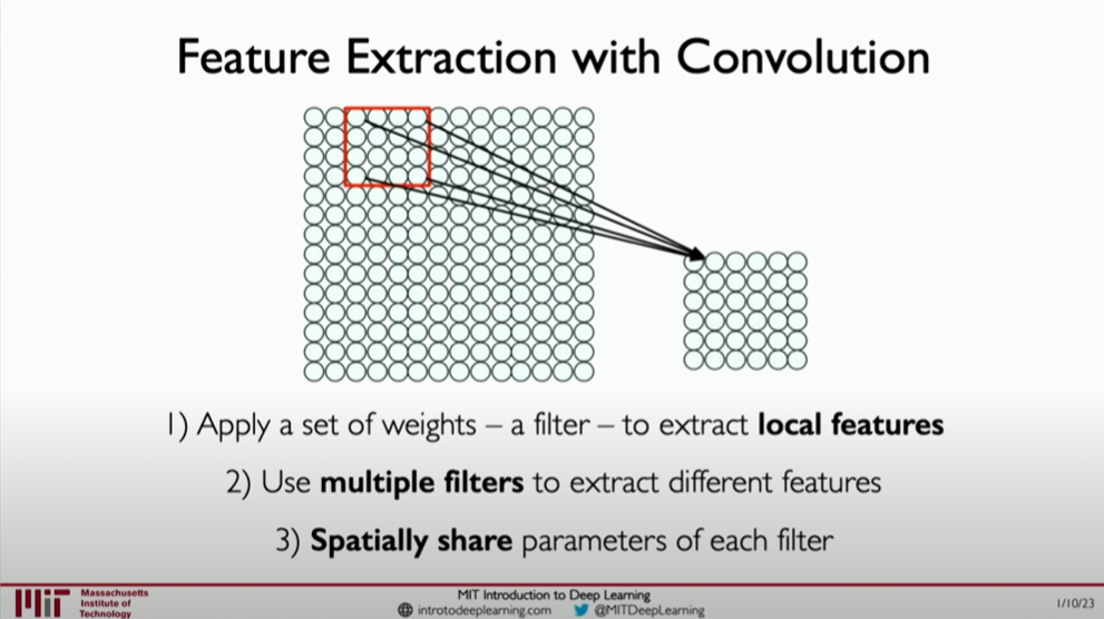
Convolutional layers operate by applying a set of learned filters (or kernels) to the input image. Each filter focuses on capturing specific patterns in the input image, such as edges, corners, or more complex textures.

• Filters: In a convolutional network, filters are small, learned matrices that are much smaller than the input image. The filter slides over the image (a process called “convolution”), performing a dot product operation at each position and summing the results to generate an output value in a new image (feature map).

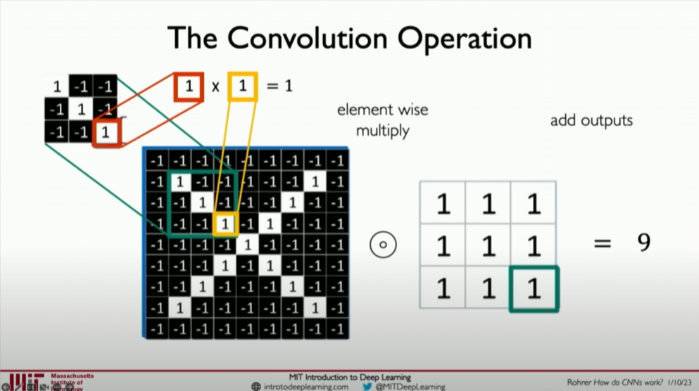
In practice, it is the dot product between two patches, and the resulting single numerical value represents the similarity between them.

• Feature Maps: The output generated by applying the filter is called a feature map, representing the extent to which the filter’s pattern is present in the input image at various locations. High values in the feature map indicate strong presence of the pattern the filter is designed to detect.

Example of Automatic Feature Extraction

Consider a simple task: recognizing the presence of a straight line in an image. We can design a filter specifically to detect the presence of a straight line. This filter will produce high response values when it detects line regions and low values elsewhere.

Producing Feature Maps

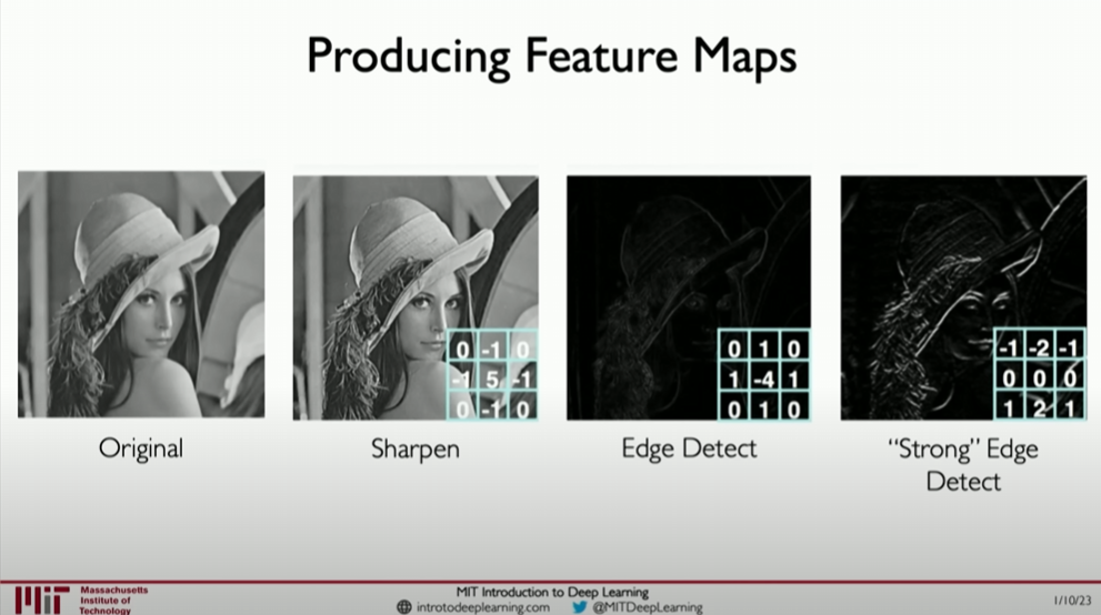
Just by slightly changing the filter weights, we can achieve drastically different results.

Example of Filters

A simple filter for detecting horizontal lines might look like this:

[[-1, -1, -1],
 [ 2,  2,  2],
 [-1, -1, -1]]

This filter is designed to detect horizontal lines. The positive values in the middle row capture the horizontal line features, while the negative values in the top and bottom rows help highlight these lines against the background.

Code Example: Building and Training a Simple CNN with TensorFlow

Here is a code example that uses Python and TensorFlow to build a simple CNN for an image classification task:

import tensorflow as tf
from tensorflow.keras.layers import Conv2D, MaxPooling2D, Flatten, Dense

model = tf.keras.Sequential([
    # Convolutional layer with 32 3x3 filters
    Conv2D(32, (3, 3), activation='relu', input_shape=(28, 28, 1)),
    # Max pooling layer with a 2x2 pooling window
    MaxPooling2D(pool_size=(2, 2)),
    # Flatten layer to convert 3D features into 1D feature vector
    Flatten(),
    # Fully connected layer with 128 neurons
    Dense(128, activation='relu'),
    # Output layer with 10 neurons corresponding to 10 categories, using softmax activation
    Dense(10, activation='softmax')
])

# Compile the model
model.compile(optimizer='adam', loss='sparse_categorical_crossentropy', metrics=['accuracy'])

# Print model summary
model.summary()

This model first uses a convolutional layer to extract basic features from the image, then reduces the spatial dimensions of these features using a pooling layer, followed by a flatten layer to convert multidimensional features into a one-dimensional vector. Finally, a fully connected layer processes these features, and the last fully connected layer (output layer) with a softmax activation function outputs the model’s predictions for 10 categories. The entire process is optimized to improve accuracy on the image classification task using the Adam optimizer and sparse categorical cross-entropy loss function.

Conclusion

Convolution and feature extraction are key to the success of CNNs in image processing tasks. By automatically learning filters from training data, CNNs can recognize complex patterns and objects in images, enabling efficient and accurate image classification. This automatic feature learning mechanism greatly simplifies image processing tasks, making manual feature design unnecessary.

Convolutional neural networks

This section further deepens the understanding of convolutional neural networks (CNNs), particularly how convolutional layers are constructed and their application in tasks such as image classification and object detection.

Basic Composition of CNNs

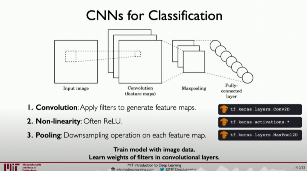
1. Convolutional Layers:

• Purpose: Convolutional layers are the core of CNNs, used to extract features from input images. They work by sliding multiple filters (also called convolution kernels or weights) over the image, performing a dot product operation with the image patch at each position.
• Filters: Each filter is designed to capture a specific feature of the image, such as edges, color changes, or more complex texture patterns. During training, the filters are automatically adjusted to better capture features useful for the classification task.

2. Activation Layers:

Use Non-linearity (non-linear activation functions) to process non-linear data.

• ReLU Activation Function: After convolutional layers, a non-linear activation function, most commonly ReLU (Rectified Linear Unit), is applied. ReLU aims to increase the network’s non-linear capability, allowing it to learn more complex features.

3. Pooling Layers:

• Purpose: Pooling layers reduce the spatial dimensions (width and height) of feature maps, decreasing the number of parameters and computational cost while preserving important information. Max pooling is the most commonly used type of pooling, which transforms each small region of the input into the maximum value in that region.

4. Fully Connected Layers:

• Classification Decision: After a series of convolution, activation, and pooling operations, the final feature maps are flattened and fed into one or more fully connected layers for the final classification decision. These layers are similar to traditional neural network layers, where each neuron is connected to all neurons in the previous layer.

Building a Convolutional Neural Network

1. Core of Convolution Operation: The convolution operation is the foundation of CNNs, allowing the extraction of local features from the input image through filters (or kernels). These features include edges, textures, and are crucial for understanding the image content.

2. Local Connections and Weight Sharing: In the convolution operation, each neuron is connected only to a small region of the input image (local connection), and the same filter is used across the entire convolutional layer (weight sharing). This design significantly reduces the number of parameters in the model while capturing the spatial hierarchy of the image.

   

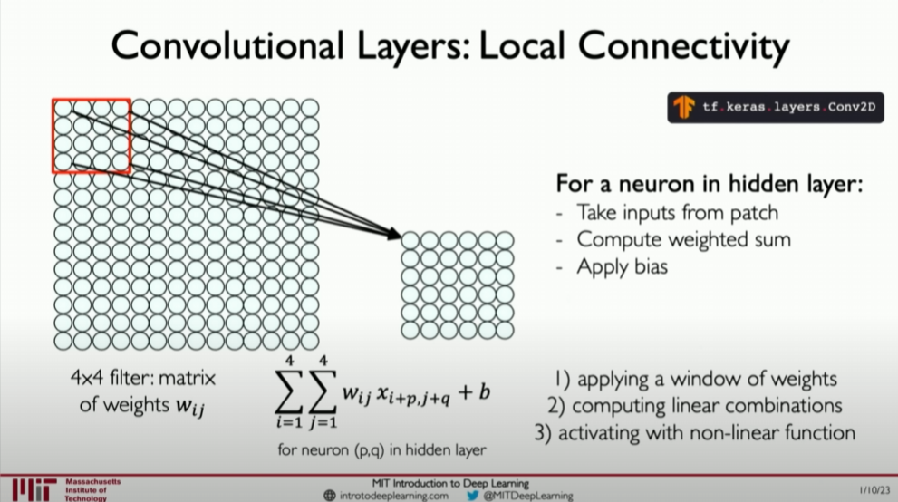
   Let’s revisit the convolution operation again, where each neuron is connected only to a small region of the input image (local connection), allowing our final model to scale to very large images.

Three Main Operations of CNNs

1. Convolutions: As described above, convolutional layers capture local features of the image through filters and generate feature maps.

2. Non-linear Activation (ReLU, etc.): Applying non-linear activation functions (such as ReLU) after the convolution operation to introduce non-linearity and increase the model’s ability to learn complex patterns. The activation function after the convolution operation enhances the model’s expressive power.

3. Pooling: Pooling layers usually follow convolutional layers to downsample the feature maps. This operation reduces the size of the feature maps, decreases computational cost, and maintains the main information. Pooling operations make the network more robust to small changes in the input image.

Spatial Arrangement of Output Volume

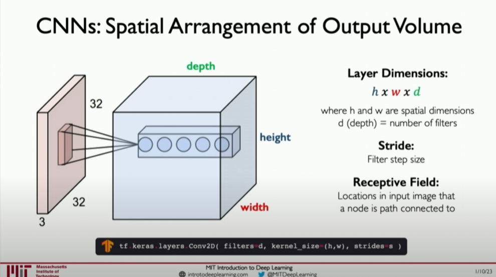
When discussing convolutional neural networks (CNNs), a crucial concept is emphasized: the ability of a single convolutional layer to detect multiple sets of features. This is particularly important when dealing with complex images, such as facial recognition, where recognizing just one feature (like an eye) is not enough. Instead, effective recognition requires detecting multiple features in the image, including eyes, nose, mouth, and ears. The combination of these features defines a face and is essential for classification.

To achieve this, CNNs output a volume of different images through convolutional operations, with each slice representing a different filter. These filters correspond to specific patterns or features that can be identified in the original input. This approach allows the network to recognize multiple features simultaneously, thereby enhancing recognition and classification accuracy.

The discussion also delves into the concept of neuron connections, particularly the concept of the receptive field, which refers to the input nodes to which a neuron is connected in the previous layer. The parameters of these connections define the spatial arrangement of information within the network, especially how it propagates through convolutional layers. Understanding how these connections are defined and how the output of a convolutional network forms a volume is critical for a deep understanding of CNNs’ workings.

Ultimately, this detailed understanding of convolutional operations and how they enable networks to recognize and process multiple features in images is central to CNNs’ core functionality. Through this approach, CNNs can achieve efficient and accurate feature

recognition and classification when handling complex images.

Example of Building a Simple CNN Architecture

Consider building a simple CNN to recognize digits in images. Our input images are 28x28 pixels grayscale images of handwritten digits, and the goal is to recognize the digit in each image (0 to 9).

Code Example: Building a Simple CNN

1. Input: 28x28 pixels grayscale images.
2. First Convolutional Layer: Use 16 3x3 filters with a stride of 1 and no padding (‘valid’). This layer aims to capture basic edges and shapes.
3. First Activation Layer: Apply the ReLU activation function.
4. First Pooling Layer: Apply 2x2 max pooling to reduce the spatial dimensions of the feature maps.
5. Second Convolutional Layer: Use 32 3x3 filters to further extract features.
6. Second Activation Layer: Apply the ReLU activation function again.
7. Second Pooling Layer: Apply 2x2 max pooling again.
8. Fully Connected Layer: Flatten the feature maps and pass them through a fully connected layer with 128 neurons to integrate features from different parts of the image.
9. Output Layer: A final fully connected layer with 10 neurons (corresponding to the 10 digit categories) using a softmax activation function to output the probability for each category.

import tensorflow as tf

model = tf.keras.models.Sequential([
    tf.keras.layers.Conv2D(16, (3, 3), activation='relu', input_shape=(28, 28, 1)),
    tf.keras.layers.MaxPooling2D(2, 2),
    tf.keras.layers.Conv2D(32, (3, 3), activation='relu'),
    tf.keras.layers.MaxPooling2D(2, 2),
    tf.keras.layers.Flatten(),
    tf.keras.layers.Dense(128, activation='relu'),
    tf.keras.layers.Dense(10, activation='softmax')
])

model.compile(optimizer='adam',
              loss='sparse_categorical_crossentropy',
              metrics=['accuracy'])

model.summary()

Summary

Convolutional neural networks automatically learn features from images through a series of convolution, non-linear activation, and pooling operations. The local connection and weight-sharing mechanisms of convolutional layers significantly reduce the complexity of the model while capturing the spatial information of the image. In this way, CNNs can effectively perform visual tasks such as image classification and object detection. Understanding and mastering these concepts are crucial for deep learning and applying it in the field of vision.

Non-linearity and pooling

Before diving into the key components of non-linearity and pooling in convolutional neural networks (CNNs), we have already understood how convolutional layers extract features from input images by applying multiple filters (convolutional kernels). Now, we will further explore how CNNs enhance their feature learning and generalization capabilities by introducing non-linear activation functions and pooling layers.

Non-linear Activation Functions

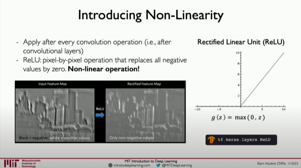
After extracting features through convolutional layers, it is crucial to introduce non-linearity using activation functions. This step aims to increase the network’s expressive power, allowing it to learn complex function mappings and capture non-linear relationships in the input data.

1. Introducing Non-linearity: After extracting feature maps from convolutional layers, the next step is to apply non-linear activation functions to these feature maps. This is because the relationships in image data are often highly non-linear, and non-linear activation functions allow the network to capture these complex relationships.

2. ReLU Activation Function: In CNNs, the most commonly used non-linear activation function is ReLU (Rectified Linear Unit). ReLU’s function is to convert all negative values to zero while keeping positive values unchanged. This simple operation helps accelerate the training process and improve the network’s convergence performance while reducing the vanishing gradient problem.

Pooling Layers

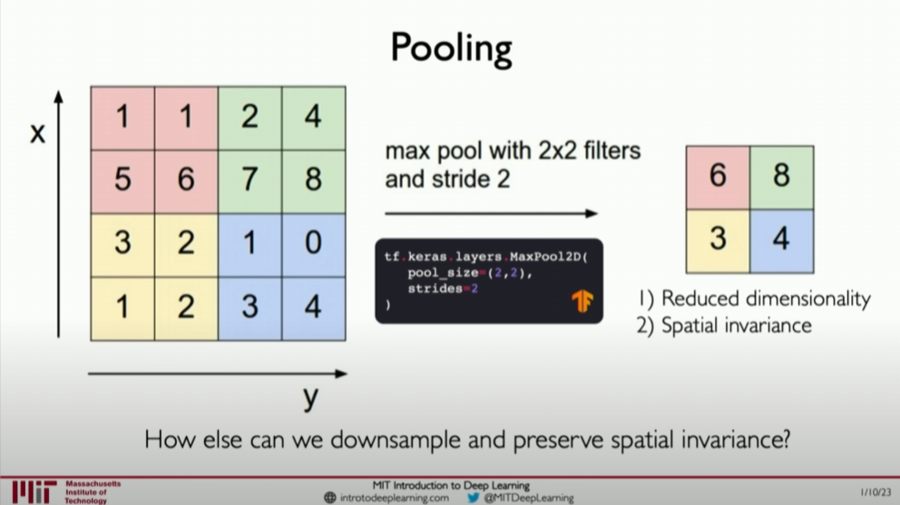
Pooling layers typically follow the ReLU activation layers and are used to reduce the spatial dimensions of the feature maps. This not only reduces the computational burden on subsequent layers but also enhances the model’s robustness to input variations.

1. Reducing Dimensionality: The primary purpose of pooling layers is to reduce the spatial dimensions (height and width) of the feature maps, thereby reducing the number of parameters in the subsequent layers and the risk of overfitting.

2. Max Pooling: The most common pooling operation is max pooling, which selects the maximum value within each small region of the input. This helps the network focus on the most prominent features and improves the model’s insensitivity to small positional changes.

3. Other Pooling Operations: Besides max pooling, there are other types of pooling operations, such as average pooling, which computes the average value within each small region. Although max pooling is more commonly used in practice, other pooling techniques can also be explored depending on the specific task requirements.

Next Steps in Building CNNs

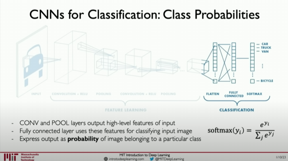
After a series of convolutional and pooling operations, the final feature maps are fed into the fully connected layers of the network. Here, the feature maps are flattened into one-dimensional arrays, and the fully connected layers utilize these flattened features to perform classification or other high-level tasks.

1. Fully Connected Layers: The task of the fully connected layers is to make the final decision (such as classification) based on the features learned from the convolutional and pooling layers. These layers are similar to traditional neural network layers, where each neuron is connected to all outputs of the previous layer.

2. Softmax Activation Function: In classification tasks, the last fully connected layer usually employs the Softmax activation function. Softmax converts the output of the fully connected layer into a probability distribution, representing the probability of each category. This makes the model’s output directly interpretable as predictions for each category.

Building a Simple CNN Model

Next, we demonstrate how to build a simple CNN for handwritten digit classification using a Python code example with TensorFlow:

import tensorflow as tf

model = tf.keras.Sequential([
    # Convolutional layer 1: 32 filters of size 3x3, ReLU activation function
    tf.keras.layers.Conv2D(32, (3, 3), activation='relu', input_shape=(28, 28, 1)),
    # Max pooling layer 1: 2x2 pool size
    tf.keras.layers.MaxPooling2D((2, 2)),
    
    # Convolutional layer 2: 64 filters of size 3x3, ReLU activation function
    tf.keras.layers.Conv2D(64, (3, 3), activation='relu'),
    # Max pooling layer 2: 2x2 pool size
    tf.keras.layers.MaxPooling2D((2, 2)),
    
    # Flatten layer: converts 2D feature maps to 1D feature vector
    tf.keras.layers.Flatten(),
    # Fully connected layer: 128 neurons, ReLU activation function
    tf.keras.layers.Dense(128, activation='relu'),
    # Output layer: 10 neurons, Softmax activation function for multi-class classification
    tf.keras.layers.Dense(10, activation='softmax')
])

# Compile the model
model.compile(optimizer='adam',
              loss='sparse_categorical_crossentropy',
              metrics=['accuracy'])

# Print model summary
model.summary()

This model first extracts image features through two convolutional and max-pooling layers, then converts these features into a one-dimensional vector through a flatten layer, and finally performs classification through fully connected layers. The ReLU activation function is used after each convolutional layer to introduce non-linearity, and max-pooling layers reduce the spatial dimensions of the feature maps.

Conclusion

By introducing non-linear activation functions and pooling layers, CNNs can effectively handle non-linear relationships in images and reduce model complexity through downsampling. These operations not only improve the network’s computational efficiency but also enhance its performance on various visual tasks. Finally, the application of fully connected layers and the Softmax activation function enables CNNs to convert learned features into specific task outputs, such as classification labels. This end-to-end process demonstrates CNNs’ powerful capabilities in handling visual tasks.

End-to-end code example

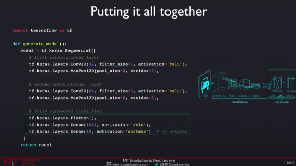
To build a fully custom convolutional neural network (CNN) from start to finish, we need to understand how to progressively stack different network layers to form an effective model. This process involves convolutional layers, pooling layers, non-linear activation layers, fully connected layers, and finally classification layers. Here are the detailed steps and code examples to build a simple CNN for image classification.

Detailed Steps to Build a CNN

1. Input Layer:
   • This is the entry point where the network receives data. For image processing tasks, the input layer shape typically matches the image dimensions. For example, for a 28x28 pixel grayscale image, the input layer shape would be (28, 28, 1).
2. Convolutional Layers:
   • **Purpose

**: Use a set of filters to extract features from the image (such as edges, corners, textures, etc.).
- Operation: Each filter slides over the input image, computing the dot product with the local region of the image to generate a feature map.
3. Activation Layers (ReLU):
- ReLU Activation Function: Converts all negative values to zero while keeping positive values unchanged. This step increases the network’s non-linear capabilities since real-world data interpretations are often non-linear.
4. Pooling Layers (Max Pooling):
- Purpose: Reduce the size of the feature maps, increasing computational efficiency while retaining important features.
- Max Pooling: Selects the maximum value within each pooling window, effectively extracting the most prominent features.
5. More Convolution and Pooling Layers:
- Typically, multiple convolution and pooling layers are used in succession to progressively extract more complex high-level features.
6. Flatten Layer:
- Converts the 2D feature maps into a 1D vector, making it suitable for fully connected layers.
7. Fully Connected Layers:
- Combine the high-level features learned to make the final classification decision.
8. Output Layer (Softmax):
- Use the Softmax activation function to convert the fully connected layer output into a probability distribution representing the prediction probabilities for each category.

Python Code Example: Building a CNN with TensorFlow

This example demonstrates how to use TensorFlow to build a CNN for MNIST digit classification:

import tensorflow as tf
from tensorflow.keras.layers import Conv2D, MaxPooling2D, Flatten, Dense, Input

# Build the model
model = tf.keras.Sequential([
    Input(shape=(28, 28, 1)),
    Conv2D(32, kernel_size=(3, 3), activation='relu'),
    MaxPooling2D(pool_size=(2, 2)),
    Conv2D(64, kernel_size=(3, 3), activation='relu'),
    MaxPooling2D(pool_size=(2, 2)),
    Flatten(),
    Dense(128, activation='relu'),
    Dense(10, activation='softmax')
])

# Compile the model
model.compile(optimizer='adam',
              loss='sparse_categorical_crossentropy',
              metrics=['accuracy'])

# Display model summary
print(model.summary())

# Train the model
# model.fit(x_train, y_train, epochs=10, validation_data=(x_test, y_test))

This code defines a CNN with two convolutional layers and two max-pooling layers, followed by two fully connected layers. This layer structure progressively extracts low- to high-level image features and finally performs classification.

Conclusion

This end-to-end CNN structure provides a complete process for automatically learning features from raw images and performing classification. By alternating convolutional and pooling layers, the network can progressively build an understanding of image content, while the fully connected layers and Softmax output layer convert these features into classification results. This not only demonstrates deep learning’s powerful capabilities in image recognition tasks but also provides a general framework that can be applied to various image processing tasks.

Applications

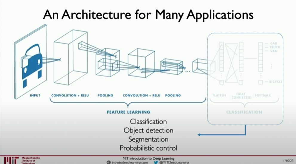
In this lecture, we explored the broad applications of convolutional neural networks (CNNs) beyond the initially discussed image classification tasks. The flexibility of CNNs’ structure and building blocks allows them to be applied to a wide range of scenarios, including but not limited to image segmentation, image captioning, and medical image analysis. Here, we will delve into CNNs’ extensibility and how to leverage this network structure for different types of tasks.

1. Flexibility of CNN Building Blocks and Applications

CNNs consist of two main parts: feature extraction and task-specific execution.

• Feature Extraction: This is the first part of CNNs, primarily using convolutional and pooling layers to learn core features from input data. These features are general and can be used for various downstream tasks.

• Task-Specific Execution: This is the second part of CNNs, usually composed of fully connected and output layers, to perform specific tasks such as classification, detection, etc.

2. Extending CNNs to Other Fields

The feature extraction part of CNNs can be viewed as a powerful feature detector that can be combined with different “heads” to perform various visual tasks:

• Image Segmentation: In image segmentation, CNNs can be trained to classify each pixel in the image into a category, commonly used in medical image processing, such as identifying tumors or other structures.

• Image Captioning: By combining recurrent neural networks (RNNs) or transformers, CNNs can generate textual descriptions of image content, useful in automatic content generation and aiding visually impaired individuals.

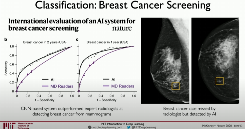
• Medical Decision Making: CNNs show great potential in medical image analysis, helping to identify disease markers, such as diagnosing from X-rays, MRIs, or CT scans.

3. Example: Extending CNNs to Medical Image Analysis

Suppose we want to design a CNN to detect brain tumors in MRI scans. The basic steps might include:

• Convolutional and Pooling Layers: Same as general image classification models, used to extract low- and mid-level features from images.

• Customized Fully Connected Layers: These layers are adjusted for specific medical analysis tasks, possibly including more regularization to handle characteristics like imbalanced and small training samples in medical data.

• Output Layer: Different from traditional classification output layers, medical image analysis might need to output more specific information, such as the size, shape, and exact location of tumors.

Code Example: Building a Medical Image Analysis CNN with TensorFlow

import tensorflow as tf
from tensorflow.keras.layers import Conv2D, MaxPooling2D, Flatten, Dense

model = tf.keras.Sequential([
    Conv2D(32, (3, 3), activation='relu', input_shape=(256, 256, 1)),
    MaxPooling2D((2, 2)),
    Conv2D(64, (3, 3), activation='relu'),
    MaxPooling2D((2, 2)),
    Flatten(),
    Dense(128, activation='relu'),
    Dense(1, activation='sigmoid')  # Assuming our task is to determine the presence of a tumor
])

model.compile(optimizer='adam',
              loss='binary_crossentropy',
              metrics=['accuracy'])

This simple model framework demonstrates how to adapt a CNN for medical image analysis, where the output layer is designed to determine whether a tumor is present in the image.

Conclusion

These examples and discussions show that the structure and building blocks of CNNs provide great flexibility, allowing them to be applied not only to image classification but also to other complex visual tasks. This extensibility makes CNNs powerful tools for processing various image data, especially in applications requiring fine feature parsing.

Object detection

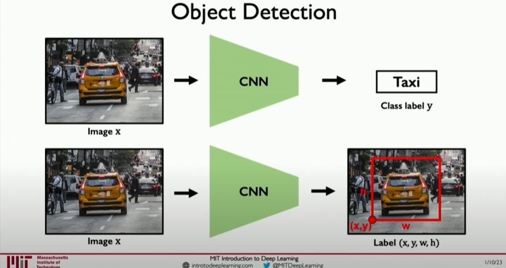
Object detection is a particularly important task in computer vision that involves two main problems: locating objects in images and identifying their categories. In this section, we explore how convolutional neural networks (CNNs) perform these tasks and mention advanced techniques for improving processing efficiency and accuracy. Object detection is crucial in many practical applications, especially those requiring precise understanding of the location of image content, such as autonomous driving and security systems. Here are the specific steps and key points of this process.

Core Problems and Challenges of Object Detection

Object detection involves not only identifying which objects exist in the image but also accurately locating these objects. This is usually achieved by predicting bounding boxes, which define the specific positions of objects in the image. This involves two main tasks:

1. Localization: Determining the location of each object in the image.
2. Classification: Identifying the category of each object.

How to Implement Object Detection

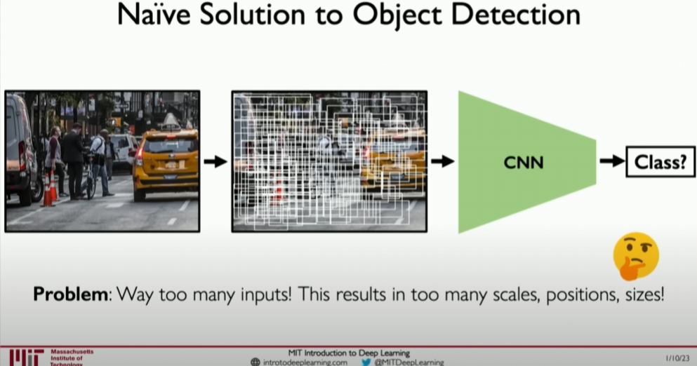
1. Generating Candidate Regions: Initially, methods would randomly or exhaustively generate multiple candidate regions, but this approach is computationally expensive and inefficient. More efficient methods use region proposal networks (RPNs), such as those used in Faster R-CNN, to intelligently generate candidate regions likely to contain objects.

2. Feature Extraction: Using convolutional layers to extract features from each candidate region. This leverages the feature learning capabilities of CNNs, converting raw pixels into higher-level abstract feature representations.

3. Bounding Box Regression: Refining the bounding boxes of each candidate region to more accurately enclose the target objects.

4. Classification: Classifying the content within each refined bounding box to determine the object category.

Advanced Model Structures

In practical applications, using more advanced model structures can address the efficiency and accuracy issues of object detection, such as:

• R-CNN (Regions with CNN features): First, multiple candidate regions are extracted from the image, and then a CNN is run on each region to extract features, followed by classifying and regressing bounding boxes.

  

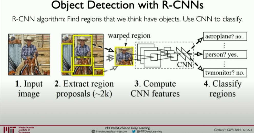
• Faster R-CNN: Builds on R-CNN by adding a region proposal network (RPN) to automatically learn to generate high-quality candidate regions in the image

, significantly improving efficiency.

Advanced Model: Faster R-CNN

Faster R-CNN is an efficient object detection framework that improves efficiency and accuracy through the following steps:

• Region Proposal Network (RPN): Automatically learns to generate high-quality candidate regions in the image.
• ROI Pooling: Converts candidate regions of different sizes into a fixed size, allowing standard fully connected layers to process them.
• Joint Training: Simultaneously learns bounding box regression and object classification, optimizing the training process and improving performance.

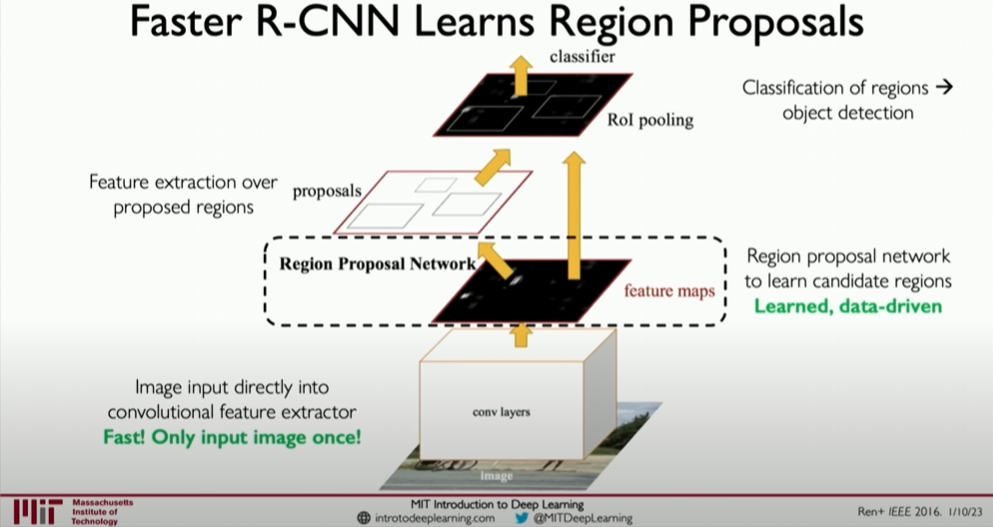
Image Segmentation: Segmentation

Alongside object detection, image segmentation is another complex but extremely important computer vision task. Image segmentation focuses on classifying every pixel in the image into the corresponding object category, achieving a precise understanding of the shape and location of each object in the image.

Core Tasks of Image Segmentation

Image segmentation is usually divided into two types: semantic segmentation and instance segmentation.

1. Semantic Segmentation: In semantic segmentation, the goal is to classify every pixel in the image so that pixels belonging to the same category are labeled as the same class. Here, different instances of the same class are not distinguished; for example, all car pixels are labeled as “car” regardless of which car they belong to.
2. Instance Segmentation: Instance segmentation not only identifies the class of each pixel but also distinguishes different instances of objects. For example, each car in the image is individually identified and labeled.

Implementing Image Segmentation

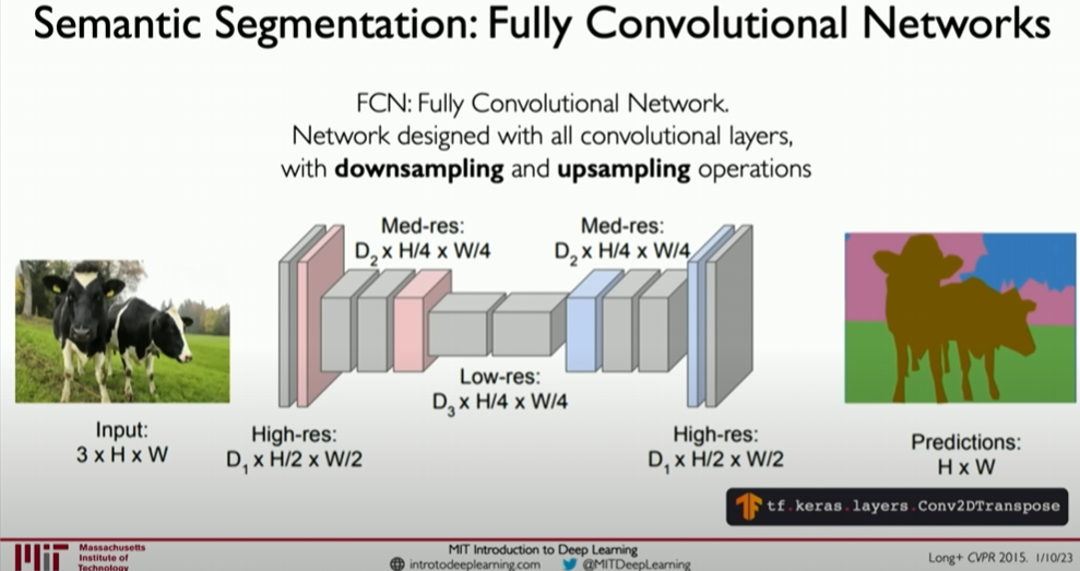
Image segmentation tasks often rely on fully convolutional networks (FCNs) or similar deep learning architectures. These networks achieve precise segmentation of images through the following steps:

1. Feature Extraction: Using convolutional layers to extract features from the raw image.
2. Downsampling: Reducing spatial resolution through pooling operations to increase the receptive field and capture broader contextual information.
3. Upsampling: Increasing the resolution of feature maps back to the original image size through deconvolution (also called transposed convolution) operations.
4. Pixel-level Classification: Classifying each pixel in the upsampled feature map to generate a segmentation map of the same size as the original image.

Example Code: Building a Simple Semantic Segmentation Model with TensorFlow

Here is a code example to build a simple semantic segmentation model using TensorFlow:

import tensorflow as tf
from tensorflow.keras.layers import Conv2D, Conv2DTranspose, MaxPooling2D

# Build a sequential model
model = tf.keras.Sequential([
    # Input layer, assuming input image size is 256x256 pixels, 3 color channels (RGB)
    tf.keras.layers.InputLayer(input_shape=(256, 256, 3)),
    
    # First convolutional layer with 32 3x3 filters, ReLU activation, same padding
    Conv2D(32, (3, 3), activation='relu', padding='same'),
    
    # First pooling layer with 2x2 max pooling window
    MaxPooling2D((2, 2)),
    
    # Second convolutional layer with 64 3x3 filters, ReLU activation, same padding
    Conv2D(64, (3, 3), activation='relu', padding='same'),
    
    # Transposed convolutional layer for upsampling, 64 3x3 filters, stride 2 (doubles feature map size)
    Conv2DTranspose(64, (3, 3), strides=(2, 2), padding='same', activation='relu'),
    
    # Final convolutional layer to produce classification output, 32 1x1 filters, softmax activation,
    # assuming 32 classes, each pixel is classified into one of 32 classes
    Conv2D(32, (1, 1), activation='softmax')
])

# Compile the model with adam optimizer, sparse categorical cross-entropy loss, and accuracy metrics
model.compile(optimizer='adam', loss='sparse_categorical_crossentropy', metrics=['accuracy'])

# Print model summary to view the architecture and parameter count
print(model.summary())

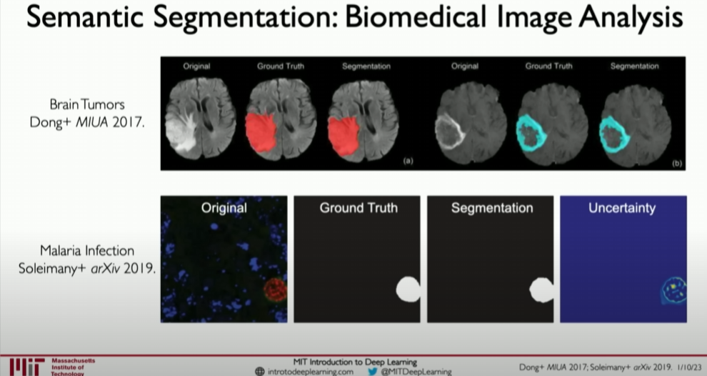
Semantic segmentation is also used in many other healthcare fields, especially for segmenting cancerous regions and even identifying malaria-infected parts in blood.

Code Example: Building a Simple Object Detection Model

Below is an example of building a simple object detection model using the TensorFlow library. This model will use convolutional layers to extract features and then use fully connected layers to predict bounding boxes and class labels.

import tensorflow as tf

# Create the model
model = tf.keras.Sequential([
    # Input layer, assuming input image size is 224x224x3
    tf.keras.layers.InputLayer(input_shape=(224, 224, 3)),
    # Convolutional and pooling layers
    tf.keras.layers.Conv2D(64, kernel_size=(7, 7), strides=(2, 2), activation='relu'),
    tf.keras.layers.MaxPooling2D(pool_size=(2, 2), strides=(2, 2)),
    # More convolution and pooling
    tf.keras.layers.Conv2D(128, kernel_size=(3, 3), activation='relu'),
    tf.keras.layers.MaxPooling2D(pool_size=(2, 2)),
    # Flatten layer for fully connected processing
    tf.keras.layers.Flatten(),
    # Fully connected layers for classification and regression
    tf.keras.layers.Dense(1024, activation='relu'),
    tf.keras.layers.Dense(4 + 1),  # Assuming 1 class and 4 coordinates (x, y, width, height)
])

# Compile the model
model.compile(optimizer='adam', loss='mse', metrics=['accuracy'])

# Print model summary
model.summary()

Conclusion

Object detection is a complex task involving multiple subtasks, including candidate region proposal, feature extraction, bounding box localization, and class classification. Advanced techniques like Faster R-CNN can significantly improve the accuracy and efficiency of object detection. The above code example demonstrates how to use common deep learning frameworks to implement a simple object detection model, providing a foundation for further learning and application.

End-to-end self-driving cars

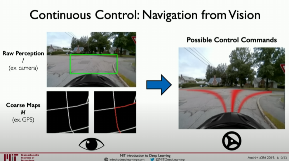
In this section, we focus on the application of autonomous driving cars, particularly how to utilize neural networks to achieve autonomous navigation. This field provides a complex yet challenging example for the application of convolutional neural networks (CNNs), as it requires not only identifying and classifying objects in images but also inferring control actions directly from images to drive the vehicle.

Key Challenges in Autonomous Driving

Autonomous driving technology aims to integrate environment perception, decision-making, and control execution into a unified system. In this case, neural networks need to process image data to classify or segment objects and output specific driving control commands, such as steering angles, speed adjustments, etc.

Neural Network Design

1. Versatility: Neural networks in autonomous driving systems are usually multifunctional. They need to accurately and quickly recognize road conditions from real-time video images while also navigating based on map data.

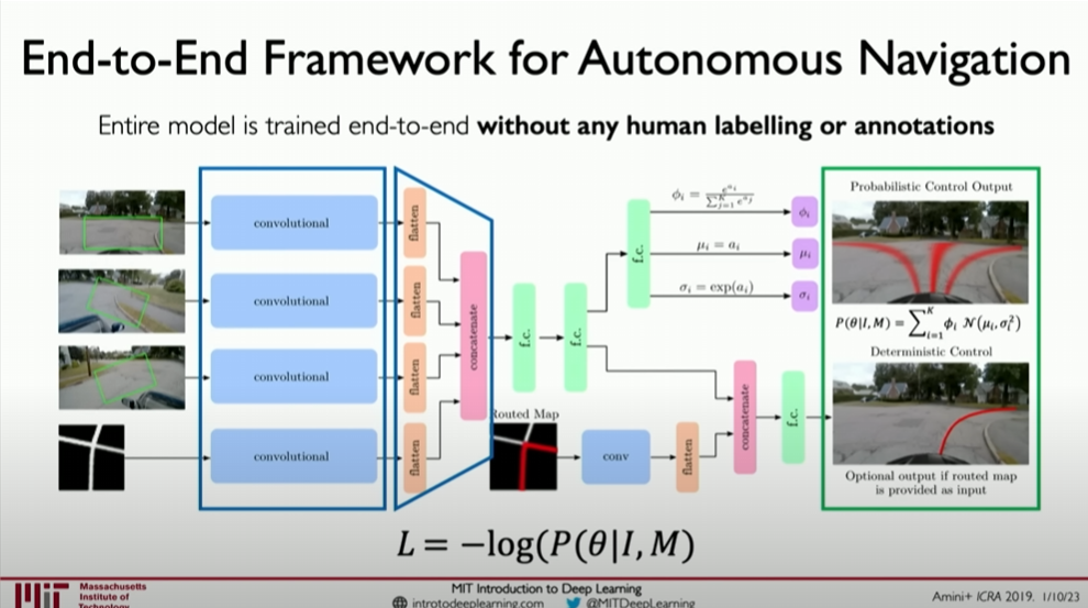
2. End-to-End Learning: From input images to output control commands, this model adopts an end-to-end learning strategy. There is no need to manually define features or encode driving rules; instead, the network learns how to respond to different road conditions from large amounts of driving data.

3. Output of Probabilistic Control Commands: In autonomous driving, the network output is not just classification labels but continuous control parameters, defining the specific actions of the vehicle, such as steering angles, acceleration, or braking. This requires the network to handle and output continuous probability distributions.

Network Structure

The network typically includes the following parts:

• Feature Extraction Layers: Using convolutional layers to identify key features in images.
• Convolutional and Pooling Layers: Extracting higher-level abstract features through multiple layers of convolution and pooling operations.
• Fully Connected Layers: Converting high-level features into control commands.

How Neural Networks Learn to Drive

1. Data Input: Input data usually includes real-time video images of the road ahead and the vehicle’s GPS position and rough map information.

   Neural networks for autonomous driving vehicles often need to process multiple forms of input data, primarily including:

   • Real-time camera video streams capturing the visual information ahead of the vehicle.
   • GPS and high-precision maps providing the vehicle’s precise position and navigation path in the environment.

2. Feature Learning: The first task of an autonomous driving neural network is to extract useful features from the video stream. This is typically achieved through multiple layers of convolutional networks, each aimed at capturing different levels of abstract features in the image data.

3. Action Inference: The extracted features are used by the decision layer to predict the best action plan for the vehicle, including steering control, speed adjustment, etc. This decision is usually based on a series of continuous probability distributions, each representing different potential actions.

4. Probabilistic Models: The output is not simple action commands but probabilistic distributions

for each possible action, allowing the vehicle to make optimal decisions amidst uncertainty, guiding the vehicle to navigate safely and effectively.

Example Code: Building a Simplified Autonomous Driving Neural Network

Assuming we use Python and the TensorFlow framework to build a simplified autonomous driving model, the following code represents a minimal version to understand basic concepts:

import tensorflow as tf
from tensorflow.keras.layers import Conv2D, Dense, Flatten, Input

# Build the model
model = tf.keras.Sequential([
    Input(shape=(224, 224, 3)),  # Assuming input image size is 224x224 RGB
    Conv2D(24, kernel_size=5, strides=2, activation='relu'),
    Conv2D(36, kernel_size=5, strides=2, activation='relu'),
    Conv2D(48, kernel_size=5, strides=2, activation='relu'),
    Conv2D(64, kernel_size=3, activation='relu'),
    Conv2D(64, kernel_size=3, activation='relu'),
    Flatten(),
    Dense(100, activation='relu'),
    Dense(50, activation='relu'),
    Dense(10, activation='relu'),
    Dense(1)  # Assuming the final output is the vehicle's steering angle
])

# Compile the model
model.compile(optimizer='adam', loss='mse')

# Model summary
model.summary()

This model takes images as input, extracts features through multiple convolutional layers, and finally predicts the vehicle’s steering angle through fully connected layers. This is just an extremely simplified example; actual autonomous driving models are far more complex, involving more input data processing and complex output strategies.

Instances and Applications

Autonomous driving car neural network models can be understood as highly complex decision systems that need to process large amounts of sensor data in real-time while ensuring the safety and reliability of decisions. By learning from large amounts of human driving data, such models can simulate human driving behavior and continually optimize to adapt to different road and traffic conditions.

This type of neural network demonstrates how deep learning can go beyond traditional task boundaries, processing multiple types of input and output through a unified framework to achieve true automation. It also highlights the powerful capabilities of deep learning technology in handling complex, high-dimensional, and dynamic environments.

Summary

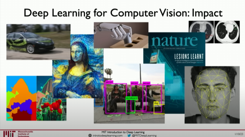
Today’s lecture delved into the broad applications and fundamental composition of convolutional neural networks (CNNs), as well as their capabilities in handling various complex tasks. Here is a summary of the lecture content:

Core Concepts and Applications

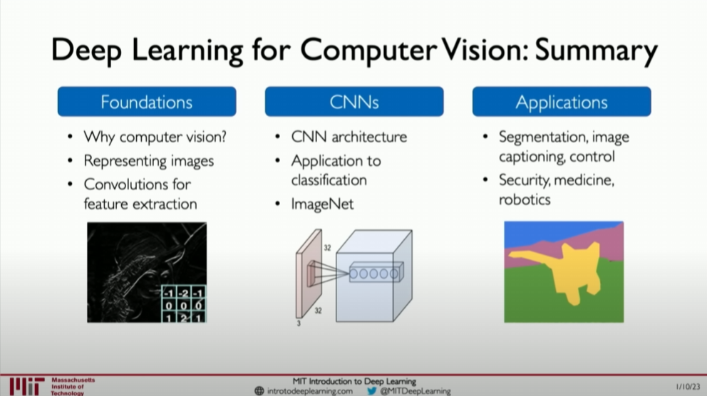
1. Convolutional Neural Networks (CNNs):

   • CNNs are powerful neural network architectures, especially suitable for image processing tasks.
   • CNNs use convolutional layers to automatically learn spatial hierarchical features from data, reducing the need for manual feature design.

2. Feature Extraction:

   • One of the key capabilities of CNNs is to extract useful features from raw data.
   • These features can then be used for various tasks such as image classification, object detection, or semantic segmentation.

3. Versatility and Flexibility:

   • A notable advantage of CNNs is their flexibility, allowing them to be adapted to different tasks by replacing the network’s “head” (the final few layers).
   • For instance, the same feature extraction base can be used for classification tasks and adapted for more complex tasks such as autonomous driving navigation.

4. Application Fields:

   • CNNs have found applications in medical image analysis, autonomous driving, facial recognition, and many other fields.
   • Their applications are not limited to simple classification tasks but extend to advanced tasks requiring precise spatial understanding and complex decision-making.

Extensions and Future Directions

• CNNs are not limited to image processing but can be extended to video analysis, natural language processing, and complex system modeling.
• With technological advancements, future CNN models will become more efficient and accurate, capable of handling larger-scale data and more complex tasks.

Course Structure

In summary, convolutional neural networks are transformative tools capable of automatically learning complex representations from images and other high-dimensional data. By effectively utilizing CNNs, we can solve problems that previously required extensive manual intervention and expertise, significantly impacting research and commercial applications across multiple fields.

---

---

---

CN

Introduction

Introduction 部分核心在于展现深度学习在计算机视觉中的应用，尤其是如何通过深度学习使计算机实现“视觉”。以下是基于该部分内容的逐步总结：

1. 课程介绍与动机：课程开始时强调了视觉作为人类最重要的感官之一的重要性，指出了人们在日常生活中极度依赖视觉来导航和理解周围世界。这部分的目的是激发兴趣，并说明深度学习在模仿这一核心人类能力方面的潜力和价值。

2. 视觉系统的目标：介绍强调了构建计算机视觉系统的终极目标不仅仅是识别物体的位置（”什么在哪里”），更重要的是理解场景的深层次含义，包括物体的动态性、预测场景中可能发生的事件等。这种能力使计算机能够更加深入地理解视觉信息，超越了表面的识别。

   

   例如上图中红绿灯的动态变化、行人的行走方向以及更多深层次的细节。

3. 深度学习的角色：通过深度学习和机器学习，我们能够构建能够“看到”和“理解”其视觉输入的系统。深度学习算法能够从原始图像数据中直接学习，无需手动编程特定的规则，这使得算法能够自动识别和学习图像中的复杂模式和特征。

4. 计算机视觉的应用示例：课程介绍中提到了多个计算机视觉应用的例子，包括自动驾驶、医疗诊断和提高无障碍技术。这些例子展示了深度学习在视觉领域的广泛应用，以及它如何推动技术革新和改善人们的生活。

5. 深度学习与计算机视觉的挑战：尽管深度学习在计算机视觉中取得了显著进展，但介绍也提到了存在的挑战，比如如何处理图像的高维数据，理解图像中的空间关系，以及如何使模型能够处理不同的视觉变化（例如光照变化、物体的移动和遮挡等）。

总结而言，这段介绍强调了计算机视觉的重要性和挑战，并介绍了深度学习如何使计算机不仅能“看到”物体，而且能深入理解视觉场景的复杂性。通过展示深度学习在各种应用中的潜力，介绍激发了学习者探索如何通过深度学习技术来构建先进的视觉系统的兴趣。

Amazing applications of vision

深度学习在计算机视觉领域的应用被详细阐述，尤其是它在推动计算机获取视觉能力方面的作用。

1. 深度学习引领革命：深度学习特别是在过去的十年中，已成为计算机视觉领域革命的主导力量。这一技术不仅促进了机器对图像的理解和处理能力的提升，而且还扩展到了日常设备，如智能手机，这些设备现在能够处理和增强拍摄的每一张图片，包括检测面部等功能。

2. 应用实例：深度学习技术在各种领域都有广泛的应用，从医学和生物学到自动驾驶车辆以及提高无障碍设施的可用性。例如，深度学习被用于医疗决策制定中，以及帮助视力障碍人士通过声音反馈导航的项目中。

   

   下面是帮助视障者跑步时预测轨迹，并进行声音提示的案例

   

3. 端到端学习模型：深度学习的一大优势在于其能力，能够直接从原始数据中学习。这意味着与传统方法相比，深度学习模型可以直接从图像中学习和提取特征，无需人工干预。这一点在特征提取任务，如面部检测和识别中尤为重要。

   

   这也会在之后的实验中进行练习

4. 自动驾驶的例子：自动驾驶是计算机视觉应用的一个重要示例。深度学习模型能够处理图像或视频输入，从而训练汽车理解其周围环境，并作出如转向、加速或制动等控制决策。这种端到端的方法与多数自动驾驶汽车公司采用的方法截然不同，展示了深度学习在处理复杂环境中的潜力。

   

5. MIT的研究项目：文中提到了MIT实验室开发的一个自动驾驶车辆项目，这一项目体现了深度学习技术在实际应用中的巨大潜力。通过学习和预测启动命令，该项目展示了如何将深度学习应用于复杂的控制系统中。

综上所述，第二部分详细描述了深度学习特别是卷积神经网络在推动计算机视觉发展方面的关键作用。从提高智能设备的图像处理能力到推动自动驾驶和医疗诊断的进步，深度学习正开辟着计算机视觉新的应用领域，并展示出改善人类生活的巨大潜力。

What computers “see”

计算机视觉的基础

在深度学习领域，计算机视觉旨在模仿人类视觉系统的功能，使计算机能够从图像或视频中识别和处理视觉信息。一个基础的例子是，当我们看到亚伯拉罕·林肯的照片时，我们可以轻易识别出人物。对计算机而言，这张照片是由大量像素组成的数字矩阵，每个像素都有一个或多个数值表示其亮度和颜色。

图像数据的数字化

• 灰度图像：每个像素由一个数字表示，该数字反映了像素的亮度或灰度级别。

  

• 彩色图像：通常使用RGB色彩模式，每个像素由三个数字组成，分别代表红色、绿色和蓝色的强度。

# 简单的Python代码片段，展示如何用数字表示一个2x2的灰度图像
gray_image = [[255, 0],
              [128, 128]]

# 对于一个2x2的RGB彩色图像
color_image = [[[255, 0, 0], [0, 255, 0]],
               [[0, 0, 255], [255, 255, 0]]]

图像处理任务

图像处理的核心任务可以分为两大类：分类（Classification）和回归（Regression）。

• 分类（Classification）：识别图像属于哪个预定义类别。例如，从一组总统的照片中识别出是哪位总统。
• 回归（Regression）：预测与图像相关的连续数值属性。例如，估计图像中对象的大小或位置。

特征提取的重要性

首先我得知道需要找什么特征（features）或者说什么模式（pattern），第二步我们需要在检测到这些模式后去推断我们现在处在哪个类别（class）

早期的计算机视觉方法依赖于手工设计的特征提取器来识别图像中的模式。但这些方法往往无法适应图像的多样性和复杂性。例如，如果我们想从不同角度拍摄的照片中识别汽车，手工设计的特征提取器可能难以覆盖所有可能的变化。

图像本质上是由数字构成的三维数组，即便是同一类别的对象，也会因为遮挡、光照变化、旋转和平移等因素出现大量变化。这使得分类任务中的分类管道需要能够处理并对这些变化保持不变性，同时对不同类别间的变化保持敏感。

然而，即使我们可以基于先验知识手动定义一些特征，这些特征面对现实世界中图像的巨大变异时，往往变得非常不稳定。这就提出了一个问题 ，我们如何构建一个既能够应对这些变异又能保持高度鲁棒性的计算机视觉算法。

解决方案：利用神经网络。神经网络能够直接从数据中学习特征，并且重要的是，它们能够层层叠加，从之前学到的特征上构建更复杂的特征集合。这样，从最基本的像素级特征到具有语义意义的特征（如人脸的眼睛和鼻子），神经网络能够以分层的方式自动提取和识别。

深度学习革命

深度学习引入了从数据中自动学习特征的概念，这一点通过使用神经网络实现。一个典型的神经网络包含多个层，每一层都能从简单的特征（如边缘和角落）自动学习到更复杂的特征（如面部或物体）。

卷积神经网络（CNN）

CNN是深度学习中用于图像处理的一类特殊网络。它们通过卷积层自动从图像中提取特征。

# 一个简单的CNN示例（使用Keras构建）
from keras.models import Sequential
from keras.layers import Conv2D

model = Sequential()
# 添加一个卷积层，输入是图像的尺寸，这里假设是28x28的灰度图像
model.add(Conv2D(filters=32, kernel_size=(3, 3), activation='relu', input_shape=(28, 28, 1)))

层次化特征学习

CNN通过其深层结构能够层次化地学习特征，从而使得模型能够识别和处理图像中的复杂模式。这种层次化的学习方式是CNN在图像分类、对象检测等任务中取得成功的关键。

总结而言，深度学习，尤其是CNN在计算机视觉领域的应用，极大地推动了这一领域的发展。通过自动从图像数据中学习特征，深度学习模型能够处理和理解从简单到复杂的各种视觉信息，为诸如自动驾驶、医疗图像分析等领域提供了强大的支持。

Learning visual features

深度学习与视觉特征

深度学习，特别是卷积神经网络（CNN），已成为图像识别和处理领域的基石。这得益于它们能够直接从原始图像数据中自动学习复杂的视觉特征，无需手动编码特征提取器。关键在于，CNN能够保持图像的空间层次结构，这对于理解图像内容至关重要。

全连接层的问题

全连接网络（fully connected network）（也称为密集网络）在图像处理任务中的主要问题在于:

图像的空间信息丢失：它们无法有效地处理图像数据的空间结构。全连接层将图像铺平为一维向量，这导致丢失图像的空间信息。例如，全连接网络难以区分排列顺序不同的像素模式，这在图像识别中是不可接受的。

参数数量的爆炸：全连接层需要处理大量参数，尤其是对于图像这种高维数据。例如，仅 100x100 像素的图像就可能导致数百万个参数，这使得模型训练变得低效且难以管理。

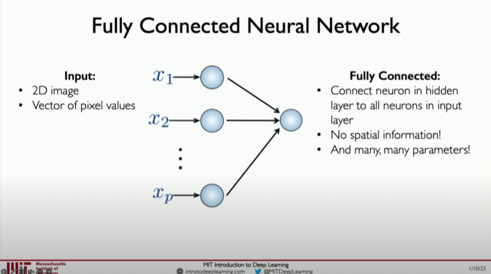
卷积神经网络（CNN）

为了克服全连接网络的局限，我们需要一种方法来保留图像的空间结构。这意味着网络的设计要能够理解和利用图像中像素之间的空间关系。

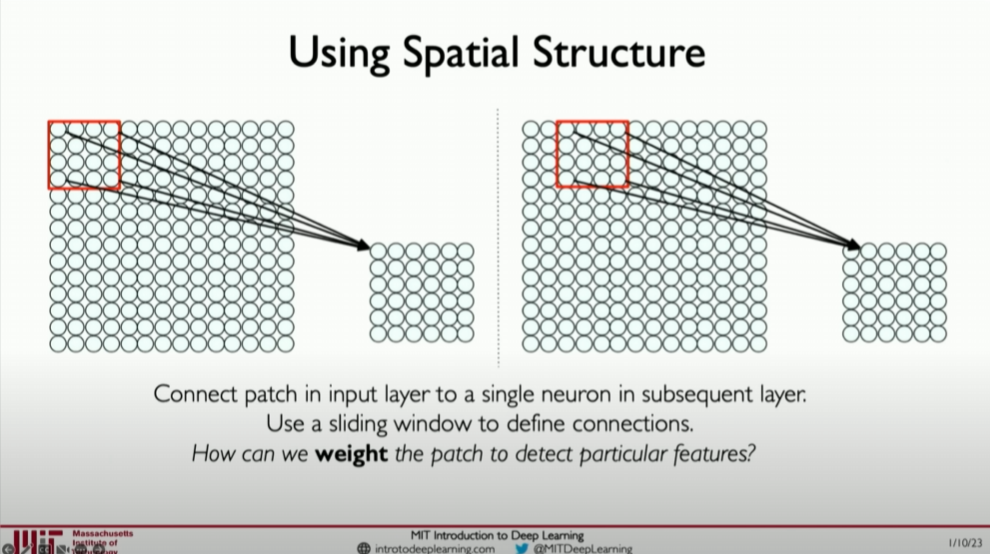
局部连接和权重共享：通过将输入图像的小块（称为“补丁（patch）”或“感受野(receptive field)”）连接到隐藏层的神经元，我们可以让每个神经元专注于图像的一小部分。这种方法不仅减少了模型的参数数量，而且允许网络学习图像中的局部模式。

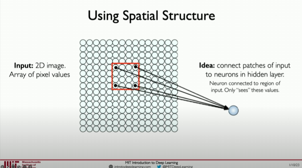
卷积层通过保持图像的空间结构来解决这个问题。它们通过在图像上滑动小窗口（称为滤波器或卷积核），在每个位置应用相同的操作来实现这一点。这种方法不仅减少了模型参数的数量（通过权重共享），而且使网络能够检测图像中的局部模式，如边缘、纹理和形状。

代码示例

下面是一个简单的CNN架构，使用Python和Keras框架构建，适用于图像分类任务：

from keras.models import Sequential
from keras.layers import Conv2D, MaxPooling2D, Flatten, Dense

model = Sequential([
    # 第一个卷积层，使用32个3x3的滤波器和ReLU激活函数
    Conv2D(32, (3, 3), activation='relu', input_shape=(64, 64, 3)),
    # 第一个池化层，使用2x2池化窗口
    MaxPooling2D(pool_size=(2, 2)),
    # 第二个卷积层，增加滤波器数量提取更复杂的特征
    Conv2D(64, (3, 3), activation='relu'),
    MaxPooling2D(pool_size=(2, 2)),
    # 展平层，将二维卷积层输出转换为一维，以便全连接层处理
    Flatten(),
    # 全连接层
    Dense(128, activation='relu'),
    # 输出层，使用softmax激活函数进行多分类
    Dense(10, activation='softmax')
])

model.compile(optimizer='adam', loss='categorical_crossentropy', metrics=['accuracy'])

这个模型是为处理 64x64 像素的彩色图像（3个颜色通道）设计的。它首先通过两个卷积层和池化层来提取图像特征，然后使用全连接层对这些特征进行分类。这种模型结构允许网络学习从简单到复杂的视觉特征，适用于各种图像识别任务。

层次化特征学习

CNN的一个关键优势在于其能力层次化学习特征。在网络的初级阶段，模型学习识别简单的视觉模式（如边缘和角落）。在更深的层中，网络能够组合这些初级特征来识别更复杂的结构（如物体部件）。最终，模型能够识别高级概念（如特定物体或场景）。

这种从原始像素到复杂概念的逐步学习过程是CNN在图像处理任务中取得显著成功的关键。通过自动从大量标注数据中学习视觉特征，深度学习模型能够在多种复杂环境中准确地识别和分类图像。

Feature extraction and convolution

深入讲解特征提取和卷积在图像处理中的核心作用，我们需要理解卷积神经网络（CNN）如何利用卷积（convolution）操作从图像中自动学习特征，进而实现图像的分类和识别。卷积操作通过滤波器（filter）（也称为卷积核）识别图像中的局部特征，这些局部特征随后可以组合成更复杂的图像表示。

卷积操作详解

卷积是一种数学运算，通过在输入图像上滑动一个小窗口（filter）（也称为滤波器或卷积核）来执行。对于每一个滤波器的位置，都会计算滤波器与其覆盖的图像区域的点积（dot product），并将结果求和以生成输出图像（特征图）的一个像素值。这个过程重复进行，直到滤波器覆盖了输入图像的所有位置。

滤波器（filter）的作用

滤波器是卷积网络中学习得到的参数。在训练过程中，网络通过反向传播算法调整滤波器的值，以便更好地捕捉输入图像中的特征。一开始，滤波器可能只能检测到简单的边缘或颜色变化。随着网络层的增加，后续层能够组合前面层的特征，以检测更复杂的图像模式。

滤波器决定了网络能够检测到的特征类型。例如，某些滤波器可能专门用于检测图像中的边缘，而另一些滤波器则可能用于检测更复杂的模式，如对角线或交叉点。

滤波器作为特征探测器：在卷积神经网络中，每个滤波器都充当一个特征探测器，专门寻找输入图像中的特定模式。通过组合多个这样的特征探测器的输出，网络能够理解和识别图像中的复杂对象。

空间不变性

一个关键的优点是卷积网络对图像中特征的位置变化具有不变性。即使图像中的对象移动或旋转，通过卷积操作提取的特征仍然可以被网络识别。这是因为无论特征出现在图像的哪个位置，滤波器都会检测到它。

实际例子：检测图像中的“X”

假设我们要设计一个卷积神经网络来识别图像中是否存在字母“X”。字母“X”可以通过两条交叉的对角线来特征化。我们可以训练网络来识别这些对角线，无论它们在图像中的位置如何。

步骤示例：

1. 初始化滤波器：开始时，我们随机初始化滤波器的权重。

2. 滑动滤波器：将每个滤波器在整个图像上滑动，计算滤波器与图像局部区域的点积。

3. 特征图生成：对于每个滤波器位置，计算结果形成一个新的图像（特征图），表示特定特征在图像中的位置。

4. 训练网络：通过训练数据训练网络，网络学习调整滤波器，以便它们可以更好地识别字母“X”的特征，如对角线和交叉点。

代码示例：

使用Python和TensorFlow构建一个简单的CNN来识别包含字母“X”的图像：

import tensorflow as tf
from tensorflow.keras import layers, models

model = models.Sequential([
    # 卷积层，识别图像中的局部特征
    layers.Conv2D(32, (3, 3), activation='relu', input_shape=(28, 28, 1)),
    # 池化层，降低特征图的空间尺寸，保留最重要的特征
    layers.MaxPooling2D((2, 2)),
    # 展平层，将二维特征图转换为一维，以供全连接层处理
    layers.Flatten(),
    # 全连接层，进一步处理特征
    layers.Dense(64, activation='relu'),
    # 输出层，分类器
    layers.Dense(2, activation='softmax')
])

model.compile(optimizer='adam',
              loss='sparse_categorical_crossentropy',
              metrics=['accuracy'])

# 模型总结
model.summary()

在这个例子中，卷积层使用 32 个 3x3 大小的滤波器来检测图像中的小局部特征。池化层则降低了这些特征的空间维度，而全连接层则负责将这些局部特征组合成全图的高级表示。

总结

通过卷积神经网络的特征提取和卷积操作，我们可以有效地从图像中学习到有用的表示信息，这为图像识别和分类等视觉任务提供了强大的工具。通过训练，网络能够自动学习到识别各种图像内容所需的最优滤波器，从而实现对复杂图像模式的高效识别。

The convolution operation

深入理解卷积操作及其在自动学习图像特征中的应用，需要从卷积神经网络（CNN）的基本工作原理说起。CNN通过一系列卷积层从输入图像中自动提取有用的特征，这些特征随后用于执行各种视觉任务，如分类、检测和分割。

卷积层的工作原理

卷积层通过在输入图像上应用一组学习得到的滤波器（或称为“卷积核”）来工作。每个滤波器专注于捕捉输入图像中的某种特定模式，如边缘、角点或更复杂的纹理。

• 滤波器：在卷积网络中，滤波器是小的、学习得到的矩阵，其大小远小于输入图像的尺寸。滤波器在图像上滑动（或称为“卷积”操作），在每个位置上应用一个点乘操作，并将结果求和，从而在新的特征图上生成一个输出值。

实际是两个patch之间的点积，再求和，得到的一个数值结果就是两者的相似度

• 特征图（Feature Maps）：应用滤波器后生成的输出称为特征图，它代表了滤波器在图像上的匹配程度。特征图上的高值表示滤波器所寻找的模式在相应的位置上有很强的存在感。

自动特征提取的示例

考虑一个简单的任务：识别图像中是否存在直线。我们可以设计一个滤波器，专门用于检测直线的存在。这个滤波器可能在检测到直线区域时产生高的响应值，在非直线区域产生低的响应值。

Producing Feature Maps

只需要稍稍改变滤波器（filter）的权重，就可以看到截然不同的实现效果

滤波器示例

一个简单的直线检测滤波器可能长这样：

[[-1, -1, -1],
 [ 2,  2,  2],
 [-1, -1, -1]]

这个滤波器设计为检测水平直线。滤波器中间的正值行捕捉水平线特征，而顶部和底部的负值行帮助在背景中凸显这些线条。

代码示例：使用Keras构建和训练CNN

让我们使用Python和Keras构建一个简单的CNN，来识别含有特定模式的图像。下面的代码示例创建了一个包含一个卷积层的简单网络，用于图像分类任务。

from keras.models import Sequential
from keras.layers import Conv2D, MaxPooling2D, Flatten, Dense

model = Sequential([
    # 卷积层，32个3x3大小的滤波器
    Conv2D(32, (3, 3), activation='relu', input_shape=(28, 28, 1)),
    # 最大池化层，2x2池化窗口
    MaxPooling2D(pool_size=(2, 2)),
    # 展平层，将3D特征转换成1D特征向量
    Flatten(),
    # 全连接层，128个神经元
    Dense(128, activation='relu'),
    # 输出层，10个神经元对应10个类别，使用softmax激活函数
    Dense(10, activation='softmax')
])

# 编译模型
model.compile(optimizer='adam', loss='sparse_categorical_crossentropy', metrics=['accuracy'])

# 输出模型概要
model.summary()

这个模型首先使用一个卷积层来提取图像中的基本特征，然后通过一个池化层减少特征图的空间尺寸，接着将多维特征展平成一维向量，以便通过一个全连接层进一步处理这些特征，最后通过另一个全连接层（输出层）并应用softmax激活函数来将模型的预测输出为10个类别的概率分布，整个过程通过编译模型时指定的Adam优化器和稀疏分类交叉熵损失函数来优化模型参数，以提高在图像分类任务上的准确率。

结论

卷积和特征提取是CNN在图像处理任务中成功的关键。通过自动从训练数据中学习到的滤波器，CNN能够识别图像中的复杂模式和对象，从而实现高效准确的图像分类。这种自动特征学习机制极大地简化了图像处理任务，使得手动特征设计变得多余。

Convolution neural networks

本部分内容进一步深化了对卷积神经网络（CNN）的理解，特别是卷积层如何构建以及它们在图像分类和对象检测任务中的应用。

CNN的基本构成

1. 卷积层（Convolutional Layers）：

• 作用：卷积层是CNN的核心，用于提取输入图像中的特征。它通过在图像上滑动多个滤波器（也称为卷积核或权重），在每个位置应用滤波器与图像片段的点积运算来工作。
• 滤波器：每个滤波器旨在捕捉图像的某种特定特征，如边缘、颜色变化或更复杂的纹理模式。在训练过程中，滤波器自动调整以更好地捕捉图像中有助于分类任务的特征。

2. 激活层（Activation Layer）：

使用 Non-linearity（非线性激活函数）处理非线性的数据

• ReLU激活函数：在卷积层之后，通常会应用一个非线性激活函数，最常用的是ReLU（Rectified Linear Unit）。ReLU的目的是增加网络的非线性能力，使其能够学习更复杂的特征。

3. 池化层（Pooling Layers）：

• 作用：池化层用于降低特征图的空间维度（宽度和高度），减少参数数量和计算量，同时保持重要信息。最大池化（Max Pooling）是最常用的池化类型，它将输入的每个小区域转换为该区域的最大值。

4. 全连接层（Fully Connected Layers）：

• 分类决策：经过一系列的卷积、激活和池化操作后，最终的特征图会被展平并送入一个或多个全连接层，以进行最终的分类决策。这些层类似于传统的神经网络层，每个神经元都与前一层的所有神经元相连。

卷积神经网络的构建

1. 卷积操作核心：卷积操作是CNN的基础，通过应用滤波器（或卷积核）到输入图像上，卷积层能够提取图像的局部特征。这些特征包括边缘、纹理等，对于理解图像内容至关重要。

2. 局部连接与权重共享：在卷积操作中，每个神经元只与输入图像的一个小区域相连接（局部连接），并且在整个卷积层中使用相同的滤波器（权重共享）。这种设计不仅显著减少了模型的参数数量，而且使得模型能够捕捉到图像的空间层次结构。

   

   让我们再一次回顾卷积操作，此处每个神经元只与输入图像的一个小区域相连接（局部连接），这使得我们最终的模型可以扩展到非常达到尺寸图象

CNN的三个主要操作

1. 卷积（Convolutions）：正如上文所述，卷积层通过滤波器捕捉图像的局部特征，并生成特征图。

2. 非线性激活（ReLU等）：应用非线性激活函数（如ReLU）是为了引入非线性，使得网络能够学习复杂的模式。在卷积操作后应用激活函数能够增加模型的表达能力。

3. 池化（Pooling）：池化层通常跟随在卷积层之后，用于进行降采样（下采样）。这一操作减小了特征图的尺寸，减少计算量，同时保持了特征的主要信息。池化操作使得网络对输入图像的小变化更加鲁棒。

Spatial Arrangement of Output Volumn

在探讨卷积神经网络（CNN）时，特别强调了一个重要概念：单个卷积层能够检测多个特征集的能力。这一点尤为关键，因为在处理复杂图像，例如人脸识别时，仅识别一个特征（如眼睛）是不够的。相反，有效的识别需要检测图像中的多种特征，包括眼睛、鼻子、嘴巴和耳朵。这些特征的组合定义了面部，并且对于分类至关重要。

为了实现这一目标，CNN通过卷积操作输出一个不同图像的体积，其中每个切片代表一种不同的滤波器。这些滤波器对应于原始输入中可以识别的特定模式或特征。这种方法允许网络同时识别多个特征，从而提高了识别和分类的精度。

讨论还涉及了神经元连接的概念，特别是感受野的概念，即神经元在上一层中连接到的输入节点的位置。这些连接的参数定义了信息在网络中的空间排列，尤其是在卷积层内的传播方式。理解这些连接如何定义以及卷积网络的输出如何形成一个体积，对于深入理解CNN的工作原理至关重要。

最终，这种对卷积操作的深入理解，以及它如何允许网络通过不同的滤波器识别和处理图像中的多个特征，构成了CNN的核心。通过这种方式，CNN能够在处理复杂图像时实现高效且精确的特征识别和分类。

构建简单CNN架构的例子

考虑一个简单的CNN，假设我们正在构建一个简单的CNN来识别图像中的数字。我们的输入图像是28x28像素的手写数字图像，目标是识别图像中的数字（0到9）。

代码示例：构建一个简单的CNN

1. 输入：28x28像素的灰度图像。
2. 第一卷积层：使用16个3x3的滤波器，步长为1，没有填充（’valid’）。这一层旨在捕捉基本的边缘和形状。
3. 第一激活层：应用ReLU激活函数。
4. 第一池化层：应用2x2最大池化，减少特征图的空间尺寸。
5. 第二卷积层：使用32个3x3的滤波器，进一步提取特征。
6. 第二激活层：再次应用ReLU激活函数。
7. 第二池化层：再次应用2x2最大池化。
8. 全连接层：展平特征图并通过一个含有128个神经元的全连接层，以整合来自图像不同部分的特征。
9. 输出层：最后一个全连接层，含有10个神经元（对应10个数字类别），并使用softmax激活函数，输出每个类别的概率。

import tensorflow as tf

model = tf.keras.models.Sequential([
    tf.keras.layers.Conv2D(16, (3, 3), activation='relu', input_shape=(28, 28, 1)),
    tf.keras.layers.MaxPooling2D(2, 2),
    tf.keras.layers.Conv2D(32, (3, 3), activation='relu'),
    tf.keras.layers.MaxPooling2D(2, 2),
    tf.keras.layers.Flatten(),
    tf.keras.layers.Dense(128, activation='relu'),
    tf.keras.layers.Dense(10, activation='softmax')
])

model.compile(optimizer='adam',
              loss='sparse_categorical_crossentropy',
              metrics=['accuracy'])

model.summary()

总结

卷积神经网络通过一系列卷积、非线性激活和池化操作自动从图像中学习特征，这些操作共同构成了CNN的基础。卷积层的局部连接和权重共享机制显著减少了模型的复杂度，同时保持了对图像空间信息的捕捉能力。通过这种方式，CNN能够有效地进行图像分类、对象检测等视觉任务。这些概念的理解和掌握，对于深入学习和应用深度学习在视觉领域至关重要。

Non-linearity and pooling

在深入讨论非线性和池化这两个卷积神经网络（CNN）的关键组成部分之前，我们已经了解了卷积层如何通过应用多个滤波器（卷积核）来提取输入图像的特征。现在，我们将进一步探索CNN如何通过引入非线性激活函数和池化层来加强其特征学习和泛化能力。

非线性激活函数

在通过卷积层提取特征之后，使用ReLU激活函数引入非线性是至关重要的一步。这一步骤的主要目的是增加网络的表达能力，使其能够学习复杂的函数映射，捕捉输入数据中的非线性关系。

1. 引入非线性：在卷积层提取特征图后，接下来的步骤是对这些特征图应用非线性激活函数。这是因为图像数据及其包含的关系通常是高度非线性的，而非线性激活函数允许网络捕捉这种复杂的非线性关系。

2. ReLU激活函数：在CNN中，最常用的非线性激活函数是ReLU（Rectified Linear Unit）。ReLU的作用是将所有负值转换为零，而保持所有正值不变。这简单的操作有助于加速训练过程，并改善网络的收敛性能，同时还能减少梯度消失的问题。

池化层

池化层通常跟在ReLU激活后的卷积层之后，用于降低特征图的空间维度。这不仅减少了后续层的计算负担，也增强了模型对输入变化的鲁棒性。

1. 降低维度：池化层的主要目的是减少特征图的空间尺寸（高度和宽度），这样做可以减少后续层所需的计算量，并减少模型的过拟合风险。

2. 最大池化：最常见的池化操作是最大池化，最大池化通过只保留每个小区域内的最大值，从而降低特征图的空间尺寸。这有助于网络专注于最显著的特征，并提高模型对小的位置变化的不敏感性。

3. 其他池化操作：除了最大池化外，还有其他类型的池化操作，如平均池化，它计算每个小区域的平均值。尽管最大池化在实践中更常用，但其他池化技术也可以根据具体任务的需求进行探索。

构建CNN的下一步

经过卷积层和池化层的一系列操作后，最终的特征图会被送入网络的全连接层。在这里，特征图会被展平为一维数组，全连接层然后利用这些展平的特征进行分类或其他高级任务。

1. 全连接层：全连接层的任务是基于从卷积和池化层学习到的特征来做出最终的决策（如分类）。这些层与传统的神经网络层类似，每个神经元与前一层的所有输出相连接。

2. Softmax激活函数：在分类任务中，最后一个全连接层通常会使用Softmax激活函数。Softmax将全连接层的输出转换为概率分布，表示每个类别的概率。这使得模型的输出可以直接解释为对各个类别的预测概率。

构建一个简单的CNN模型

接下来，我们通过Python代码示例展示如何使用TensorFlow构建一个简单的CNN来执行手写数字分类任务：

import tensorflow as tf

model = tf.keras.models.Sequential([
    # 卷积层1: 32个3x3滤波器，ReLU激活函数
    tf.keras.layers.Conv2D(32, (3, 3), activation='relu', input_shape=(28, 28, 1)),
    # 最大池化层1: 2x2池
    tf.keras.layers.MaxPooling2D((2, 2)),
    
    # 卷积层2: 64个3x3滤波器，ReLU激活函数
    tf.keras.layers.Conv2D(64, (3, 3), activation='relu'),
    # 最大池化层2: 2x2池
    tf.keras.layers.MaxPooling2D((2, 2)),
    
    # 展平层: 将特征图转换为一维向量
    tf.keras.layers.Flatten(),
    # 全连接层: 128个神经元，ReLU激活函数
    tf.keras.layers.Dense(128, activation='relu'),
    # 输出层: 10个神经元，Softmax激活函数
    tf.keras.layers.Dense(10, activation='softmax')
])

# 编译模型
model.compile(optimizer='adam',
              loss='sparse_categorical_crossentropy',
              metrics=['accuracy'])

# 输出模型摘要
model.summary()

这个模型首先通过两个卷积层和最大池化层来提取图像特征，然后通过一个全连接层来整合这些特征，并最终通过一个含有Softmax激活函数的输出层来进行分类。ReLU激活函数在每个卷积层后使用，以引入非线性，而最大池化层则用于减小特征图的空间尺寸。

结论

通过非线性激活函数和池化层的引入，CNN能够有效处理图像中的非线性关系，并通过降采样来减少模型的复杂度。这些操作不仅提高了网络的计算效率，还有助于提升模型在各种视觉任务上的表现。最终，全连接层和Softmax激活函数的应用使得CNN能够将学习到的特征转换为

具体的任务输出，如分类标签。这种从原始图像到特征学习，再到任务输出的整个流程，展示了CNN在处理视觉任务中的强大能力。

End-to-end code example

要构建一个从头到尾完全自定义的卷积神经网络（CNN），我们需要明白如何逐步堆叠不同的网络层以形成一个有效的模型。这个过程不仅涉及卷积层和池化层，还包括非线性激活层（non-linearity layer）、全连接层（fully connected layer），以及最终的分类层（classification layer）。以下是对整个过程的详细步骤和代码示例，用于构建一个用于图像分类的简单CNN。

构建一个CNN的详细步骤

1. 输入层：
   • 这是网络接收数据的入口。对于图像处理任务，输入层的形状通常与图像的尺寸相匹配。例如，如果我们处理的是28x28像素的灰度图像，则输入层的形状将是 (28, 28, 1)。
2. 卷积层：
   • 目的：使用一组滤波器提取图像中的特征（如边缘、角点、纹理等）。
   • 操作：每个滤波器在输入图像上滑动，计算滤波器与图像的局部区域之间的点积，生成特征图。
3. 激活层（ReLU）：
   • ReLU激活函数：将所有负值置为零，保留正值。这一步是为了增加网络的非线性，因为真实世界的数据解释往往是非线性的。
4. 池化层（Max Pooling）：
   • 目的：减少特征图的尺寸，提高计算效率，同时保持重要的特征。
   • 最大池化：在每个池化窗口中选择最大值，有效地提取最显著的特征。
5. 更多的卷积和池化层：
   • 通常会有多个卷积和池化层交替出现，逐渐提取更复杂的高级特征。
6. 展平层：
   • 将二维特征图转换为一维，使其可以被全连接层处理。
7. 全连接层：
   • 这些层将学习到的高级特征组合起来，进行最终的分类决策。
8. 输出层（Softmax）：
   • 使用Softmax激活函数将全连接层的输出转换为概率分布，这些概率对应于每个类别的预测概率。

Python代码示例：基于TensorFlow构建CNN

这个例子演示了如何使用TensorFlow构建用于MNIST数字分类的CNN：

import tensorflow as tf
from tensorflow.keras.layers import Conv2D, MaxPooling2D, Flatten, Dense, Input

# 构建模型
model = tf.keras.Sequential([
    Input(shape=(28, 28, 1)),
    Conv2D(32, kernel_size=(3, 3), activation='relu'),
    MaxPooling2D(pool_size=(2, 2)),
    Conv2D(64, kernel_size=(3, 3), activation='relu'),
    MaxPooling2D(pool_size=(2, 2)),
    Flatten(),
    Dense(128, activation='relu'),
    Dense(10, activation='softmax')
])

# 编译模型
model.compile(optimizer='adam',
              loss='sparse_categorical_crossentropy',
              metrics=['accuracy'])

# 显示模型摘要
print(model.summary())

# 训练模型
# model.fit(x_train, y_train, epochs=10, validation_data=(x_test, y_test))

这段代码定义了一个CNN，其中包括两个卷积层和两个最大池化层，以及两个全连接层。这种层次结构能够逐步提取从低级到高级的图像特征，并最终进行分类。

结论

这种端到端的CNN结构提供了一个完整的流程，用于从原始图像中自动学习特征并进行分类。通过交替的卷积和池化层，网络能够逐步构建对图像内容的理解，而全连接层和Softmax输出层则将这些特征转化为分类结果。这不仅展示了深度学习在图像识别任务中的强大能力，也提供了一个通用的框架，可应用于各种图像处理任务。

Applications

在这段讲述中，我们探讨了卷积神经网络（CNN）的应用范围远远超出了最初讨论的图像分类任务。CNN的结构和构建块的灵活性使得它们可以适用于广泛的应用场景，包括但不限于图像分割、图像字幕和医疗图像分析。下面我们将详细分析CNN的这种扩展性以及如何利用这种网络结构来处理不同类型的任务。

1. CNN的构建块和应用的灵活性

CNN主要由两部分组成：特征提取和分类（或其他任务）执行。

• 特征提取（feature extraction）：这是CNN的第一部分，主要通过卷积层和池化层来学习输入数据的核心特征。这些特征对于网络来说是通用的，可以用于多种不同的下游任务。

• 分类或其他任务（classification）：这是CNN的第二部分，通常由全连接层和输出层组成，用于根据提取的特征来执行特定任务，如分类、检测等。

2. 扩展CNN到其他领域

CNN的第一部分（特征提取）可以被视为一个功能强大的特征检测器，可以与不同的“头部”结合，以执行多种视觉任务：

• 图像分割：在图像分割中，CNN可以被训练来识别图像中每个像素属于的类别，这常用于医学图像处理，如识别肿瘤或其他结构。

• 图像字幕：结合递归神经网络（RNN）或变压器（Transformer），CNN可以用于生成描述图像内容的文本，这在自动内容生成和辅助视觉障碍人士中非常有用。

• 医疗决策：CNN在医疗图像分析方面显示出了巨大潜力，能够帮助识别疾病标志，比如通过分析X光片、MRI或CT扫描来辅助诊断。

3. 示例：扩展CNN到医疗图像分析

假设我们要设计一个用于检测MRI扫描中脑肿瘤的CNN。基本步骤可能包括：

• 卷积和池化层：与通用图像分类模型相同，用于提取图像的低级和中级特征。

• 定制的全连接层：这些层会针对特定的医学分析任务进行调整，可能包括更多的正则化来处理医疗数据的特点，如不平衡和少量的训练样本。

• 输出层：不同于传统分类的输出层，医疗图像分析可能需要输出更具体的信息，例如肿瘤的大小、形状和确切位置。

代码示例：使用TensorFlow构建医疗图像分析CNN

import tensorflow as tf
from tensorflow.keras.layers import Conv2D, MaxPooling2D, Flatten, Dense

model = tf.keras.Sequential([
    Conv2D(32, (3, 3), activation='relu', input_shape=(256, 256, 1)),
    MaxPooling2D((2, 2)),
    Conv2D(64, (3, 3), activation='relu'),
    MaxPooling2D((2, 2)),
    Flatten(),
    Dense(128, activation='relu'),
    Dense(1, activation='sigmoid')  # 假设我们的任务是判断图像中是否存在肿瘤
])

model.compile(optimizer='adam',
              loss='binary_crossentropy',
              metrics=['accuracy'])

这个简单的模型框架展示了如何将CNN用于医疗图像分析，其中的输出层被设计为判断图像中是否存在肿瘤。

结论

通过这些例子和讨论，我们看到CNN的结构和构建块提供了极大的灵活性，使其不仅能应用于图像分类，还能扩展到其他复杂的视觉任务中。这种扩展性使得CNN成为处理各种图像数据的强大工具，尤其是在需要精细特征解析的应用场景中。

Object detection

对象检测是一个在计算机视觉领域中尤其重要的任务，涉及到两个主要问题：定位图像中的对象，并且识别这些对象的类别。在这一部分讲述中，我们探讨了如何通过卷积神经网络（CNN）来执行这些任务，并提及了如何提高处理效率和精度的高级技术。对象检测在很多实际应用中，尤其是那些需要精确理解图像内容位置的场合（如自动驾驶、安防系统等），都非常重要。以下是对这一过程的具体步骤和技术要点的解析。

对象检测的核心问题与挑战

对象检测不仅仅是识别图像中存在哪些对象，更重要的是精确地标定出这些对象的位置。这通常通过预测边界框（bounding boxes）来实现，边界框定义了对象在图像中的具体位置。这涉及到两个主要的任务：

1. 定位（Localization）：确定图像中每个对象的位置。
2. 分类（Classification）：识别每个对象的类别。

如何实现对象检测

1. 生成候选区域：首先，最初的方法是随机或穷举生成多个候选区域，但这种方法计算成本高且效率低。更高效的方法是使用区域提议网络（Region Proposal Networks, RPN），如在Faster R-CNN中使用，来智能生成可能包含对象的候选区域。

2. 特征提取：使用卷积层提取每个候选区域的特征。这是利用CNN的特征学习能力，把原始像素转换为更高级的抽象特征表示。

3. 边界框回归：对每个候选区域进行边界框的精确调整，使其更紧密地框住目标对象。

4. 分类：对调整后的每个边界框内的图像进行分类，确定它包含的对象类别。

高级模型结构

在实际应用中，使用更高级的模型结构来解决对象检测的效率和精度问题，例如：

• R-CNN（Regions with CNN features）：首先从图像中提取多个候选区域，然后对每个区域运行CNN来提取特征，最后对这些特征进行分类和边界框回归。

  

• Faster R-CNN：在R-CNN的基础上增加了区域提议网络（Region Proposal Network, RPN），这使得候选区域的生成也通过学习来进行，大大提高了效率。

高级模型：Faster R-CNN

Faster R-CNN 是一个高效的对象检测框架，它通过以下步骤来提高对象检测的效率和精度：

• 区域提议网络（RPN）：自动学习在图像中生成高质量的候选区域。
• ROI Pooling：将不同大小的候选区域转换为固定大小，以便可以使用标准的全连接层处理。
• 联合训练：同时学习边界框回归和对象分类，这优化了训练过程并提高了性能。

图像分割：segmentation

在讨论对象检测的同时，我们也接触了图像分割（segmentation），这是另一种复杂但极其重要的计算机视觉任务。图像分割主要关注如何将图像中的每个像素分类到对应的对象类别，从而实现对图像中每个物体形状和位置的精确理解。

图像分割的核心任务

图像分割通常分为两种类型：语义分割和实例分割。

1. 语义分割（Semantic Segmentation）：在语义分割中，目标是对图像中的每个像素进行分类，使得属于同一类别的像素被标记为同一类。这里不区分不同物体的实例，即图像中的所有汽车像素都被标记为“汽车”，不论它们属于哪辆汽车。
2. 实例分割（Instance Segmentation）：实例分割不仅要识别像素的类别，还需要区分不同的对象实例。例如，图像中的每辆汽车都被单独区分并标记。

图像分割的实现

图像分割任务通常依赖于全卷积网络（FCN，Fully Convolutional Network）或其他类似的深度学习架构。这些网络通过以下步骤实现图像的精确分割：

1. 特征提取：使用卷积层从原始图像中提取特征。
2. 下采样：通过池化操作减少空间分辨率，增加感受野，帮助模型捕捉更大范围的上下文信息。
3. 上采样：通过反卷积（也称为转置卷积）操作将特征图的分辨率增加到与原始图像相同的大小。
4. 像素级分类：对上采样后的特征图的每个像素进行分类，生成与原图同尺寸的分割图。

示例代码：使用 TensorFlow 构建简单的语义分割模型

以下是使用TensorFlow构建简单语义分割模型的代码示例：

import tensorflow as tf
from tensorflow.keras.layers import Conv2D, Conv2DTranspose, MaxPooling2D

# 构建一个顺序模型
model = tf.keras.Sequential([
    # 输入层，设定输入图像的形状为256x256像素，3个颜色通道（RGB）
    tf.keras.layers.InputLayer(input_shape=(256, 256, 3)),
    
    # 第一个卷积层，使用32个3x3的滤波器，激活函数为ReLU，边界填充方式为same（输入输出尺寸相同）
    Conv2D(32, (3, 3), activation='relu', padding='same'),
    
    # 第一个池化层，使用2x2的窗口进行最大池化，减少特征图的维度，增大感受野
    MaxPooling2D((2, 2)),
    
    # 第二个卷积层，使用64个3x3的滤波器，激活函数为ReLU，边界填充方式为same
    Conv2D(64, (3, 3), activation='relu', padding='same'),
    
    # 反卷积层（转置卷积），用于上采样特征图，使用64个3x3的滤波器，步长为2（特征图尺寸翻倍）
    Conv2DTranspose(64, (3, 3), strides=(2, 2), padding='same', activation='relu'),
    
    # 最后的卷积层，用于产生分类输出，使用32个1x1的滤波器，激活函数为softmax，
    # 假设有32个类别，每个像素将被分类到32个类别中的一个
    Conv2D(32, (1, 1), activation='softmax')
])

# 编译模型，使用adam优化器，损失函数为稀疏分类交叉熵，评估指标为准确度
model.compile(optimizer='adam', loss='sparse_categorical_crossentropy', metrics=['accuracy'])

# 打印模型概要，查看模型的架构和参数量
print(model.summary())

Semantic Segmentation 也被用在其他很多医疗保健领域，特别是用于分割癌症领域，甚至是识别血液中感染疟疾的部分

代码示例：构建简单的对象检测模型

下面是一个构建简单对象检测模型的例子，使用TensorFlow库。这个模型将会使用卷积层来提取特征，然后使用全连接层来预测边界框和类别标签。

import tensorflow as tf

# 创建模型
model = tf.keras.Sequential([
    # 输入层，假设输入图像尺寸为 224x224x3
    tf.keras.layers.InputLayer(input_shape=(224, 224, 3)),
    # 卷积层和池化层
    tf.keras.layers.Conv2D(64, kernel_size=(7, 7), strides=(2, 2), activation='relu'),
    tf.keras.layers.MaxPooling2D(pool_size=(2, 2), strides=(2, 2)),
    # 再次卷积和池化
    tf.keras.layers.Conv2D(128, kernel_size=(3, 3), activation='relu'),
    tf.keras.layers.MaxPooling2D(pool_size=(2, 2)),
    # 展平层，准备进行全连接处理
    tf.keras.layers.Flatten(),
    # 全连接层用于分类和回归
    tf.keras.layers.Dense(1024, activation='relu'),
    tf.keras.layers.Dense(4 + 1),  # 假设有1个类别和4个坐标（x, y, width, height）
])

# 编译模型
model.compile(optimizer='adam', loss='mse', metrics=['accuracy'])

# 打印模型概要
print(model.summary())

结论

对象检测是一项复杂的任务，涉及多个子任务，包括候选区域提议、特征提取、边界框定位和类别分类。使用高级技术如Faster R-CNN可以有效提高对象检测的精确度和效率。通过上述代码示例，我们展示了如何使用常见的深度学习框架来实现一个简单的对象检测模型，这为进一步的学习和应用提供了基础。

End-to-end self driving cars

在这段讨论中，我们关注了自动驾驶汽车的应用，尤其是如何利用神经网络来实现自主导航的问题。这一领域对于卷积神经网络（CNN）的应用提供了一个复杂但极具挑战性的范例，因为它不仅需要识别和分类图像中的对象，更需要从图像中直接推断控制车辆行驶的动作。

自动驾驶的关键挑战

自动驾驶技术试图将车辆的环境感知、决策制定和控制执行整合到一个统一的系统中。在这种情况下，神经网络不仅要处理图像数据进行分类或分割，还需要能够基于这些数据输出具体的驾驶控制指令，如转向角度、速度调整等。

神经网络的设计

1. 多功能性: 自动驾驶系统中的网络通常是多功能的。它需要从输入的实时视频图像中快速精确地识别路面情况，同时还要根据地图数据进行导航。

2. 端到端学习: 从输入图像到输出控制命令，这种模型采用端到端的学习策略。不需要手动定义特征或编码驾驶规则，而是让网络自己从大量的驾驶数据中学习如何响应不同的路况。

3. 概率控制命令的输出: 在自动驾驶中，网络输出的不仅是分类标签，更是连续的控制参数，这些参数定义了车辆的具体操作，如转向角度、加速或制动等。这需要网络能够处理和输出连续的概率分布，像下图右侧中的那样。

网络结构

网络通常包含以下部分：

• 特征提取层: 使用卷积层来识别图像中的关键特征。
• 卷积层和池化层: 通过多层卷积和池化操作，逐步提取更高层的抽象特征。
• 全连接层: 将高层特征转换为控制命令。

神经网络如何学习驾驶

1. 数据输入: 输入数据通常是车辆前方的道路视频以及车辆的GPS位置和粗略地图信息。

   自动驾驶车辆的神经网络通常需要处理多种形式的输入数据。主要包括:

   • 实时摄像头视频流，捕捉车辆前方的视觉信息。
   • GPS和高精度地图，提供车辆在环境中的精确位置和导航路径。

2. 特征学习:从视频流中提取有用的特征是自动驾驶神经网络的首要任务。这通常通过多层卷积网络实现，每一层都旨在捕捉图像数据中的不同层次的抽象特征。

3. 行动推断: 提取的特征用于决策层，以预测车辆的最佳行动方案。这包括转向控制、速度调整等。此决策通常基于一系列连续的概率分布，每个分布代表不同的潜在操作。

4. 概率模型: 输出不是简单的动作指令，而是针对每种可能动作的概率分布，使车辆能够在不确定性中做出最优决策，指导车辆如何安全有效地导航。

示例代码：构建简化的自动驾驶神经网络

假设我们使用Python和TensorFlow框架来构建一个简化的自动驾驶模型。以下代码是一个极简版本，主要用于理解基本概念：

import tensorflow as tf
from tensorflow.keras.layers import Conv2D, Dense, Flatten, Input

# 构建模型
model = tf.keras.Sequential([
    Input(shape=(224, 224, 3)),  # 假设输入图像大小为224x224 RGB
    Conv2D(24, kernel_size=5, strides=2, activation='relu'),
    Conv2D(36, kernel_size=5, strides=2, activation='relu'),
    Conv2D(48, kernel_size=5, strides=2, activation='relu'),
    Conv2D(64, kernel_size=3, activation='relu'),
    Conv2D(64, kernel_size=3, activation='relu'),
    Flatten(),
    Dense(100, activation='relu'),
    Dense(50, activation='relu'),
    Dense(10, activation='relu'),
    Dense(1)  # 假设最终输出是车辆的转向角度
])

# 编译模型
model.compile(optimizer='adam', loss='mse')

# 模型概述
model.summary()

这个模型以图像作为输入，通过多个卷积层来提取特征，最终通过全连接层输出预测的车辆转向角度。这只是一个极其简化的例子，实际的自动驾驶模型将远比这更复杂，包括更多的输入数据处理和复杂的输出策略。

实例和应用

自动驾驶汽车的神经网络模型可以理解为一个高度复杂的决策系统，它需要实时处理大量的传感器数据，同时还要确保决策的安全性和可靠性。通过学习大量的人类驾驶数据，这样的模型能够模拟人类的驾驶行为，并不断优化以适应不同的道路和交通情况。

这种类型的神经网络展示了深度学习在实际应用中如何超越传统的任务边界，通过一个统一的框架来处理多种类型的输入和输出，实现真正意义上的自动化

。这也突显了深度学习技术在处理复杂、高维度和动态环境中的强大能力。

Summary

今天的讲座深入探讨了卷积神经网络（CNN）的广泛应用和基本构成，以及它们如何被用于处理各种复杂任务的能力。以下是对整个讲座内容的总结：

核心概念和应用

1. 卷积神经网络（CNN）:

   • CNN是强大的神经网络架构，特别适用于图像处理任务。
   • CNN通过使用卷积层来自动从数据中学习空间层级特征，减少了对手动特征设计的需求。

2. 特征提取:

   • CNN的关键能力之一是从原始数据中提取有用的特征。
   • 这些特征然后可以用于多种不同的任务，如图像分类、物体检测或语义分割。

3. 多功能性和灵活性:

   • CNN的一个显著优势是其灵活性，可以通过替换网络的“头部”（后几层）来适应不同的任务。
   • 例如，相同的特征提取基础可以用于分类任务，也可以调整用于更复杂的任务，如自动驾驶车辆的导航。

4. 应用领域:

   • CNN在医疗影像分析、自动驾驶、面部识别和许多其他领域中都找到了应用。
   • 它们的应用不限于简单的分类任务，还扩展到了需要精确空间理解和复杂决策的高级任务。

扩展和未来方向

• CNN不仅局限于图像处理，还可扩展至视频分析、自然语言处理和复杂系统建模等领域。
• 随着技术的进步，未来的CNN模型将更加高效和准确，能够处理更大规模的数据和更复杂的任务。

课程结构

总之，卷积神经网络是一种极具变革性的工具，能够从图像和其他高维数据中自动学习复杂的表示。通过有效利用CNN，我们可以解决以前需要大量手工干预和专业知识的问题，这对多个领域的科研和商业应用都有深远影响。