Deep Generative Modeling

EN

Introduction

Introduction: Overview of Generative Modeling

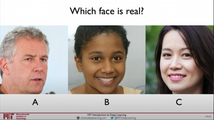
The three people in the image are all generated, none of them are real.

Course Overview

In this lecture, we will discuss the concept of Generative Models or Generative AI. In recent years, Generative AI has become a hot topic, attracting widespread attention and discussion. In this lecture, we will delve into the fundamentals of generative modeling, exploring its core idea: building systems that can not only recognize data patterns and make decisions but also generate new data instances based on learned patterns.

Definition of Generative Modeling

At its core, generative modeling involves constructing a system capable of simulating data distributions and generating new data. Generative models are not limited to traditional supervised learning; they focus on unsupervised learning. In unsupervised learning, the goal is not to learn a mapping from input to output , but to analyze the input data itself and learn its underlying patterns and features.

Supervised Learning vs. Unsupervised Learning

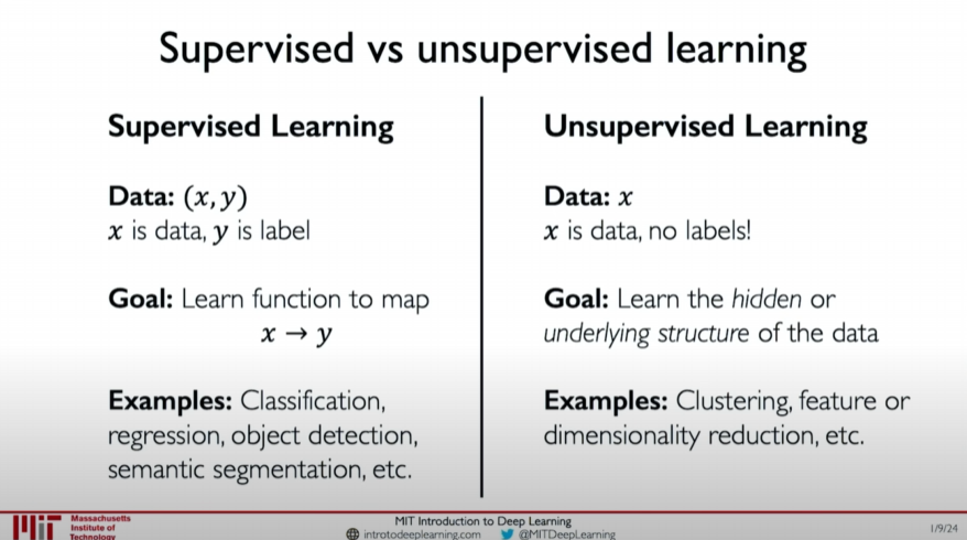
1. Supervised Learning
   • Labeled data: Each instance is accompanied by a label.
   • Goal: Learn the mapping between input data and labels.
   • Applications: Classification, regression, segmentation, etc.
2. Unsupervised Learning
   • Unlabeled data: Only input data is available, with no explicit labels.
   • Goal: Learn the underlying structure and patterns in the data.
   • Applications: Density estimation, clustering, etc.

Implementation of Generative Models

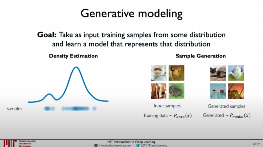
Generative models are primarily implemented in two ways:

1. Density Estimation

   • Learn and fit the probability distribution of data.
   • Goal: Find a model to simulate the probability distribution of the data.

2. Sample Generation

   • Draw new samples from the learned probability distribution.
   • Goal: Generate new data instances using the learned probability distribution.

The commonality between these two use cases of generative modeling is how we train a very good probability distribution model that resembles the true probability distribution of our real data.

Applications of Generative Modeling

Generative models have broad applications, not limited to generating realistic human faces. They play an important role in various fields, such as:

• Image generation
• Text generation
• Music generation

Course Example: Generating Fake Faces

In this lecture, we will explore how to generate realistic human face images using generative models like StyleGAN. StyleGAN is a type of Generative Adversarial Network (GAN) capable of generating high-quality, realistic images. Through these examples, we will gain a deeper understanding of the working principles and implementation methods of generative models.

Conclusion

Generative modeling is a powerful technical framework centered on learning and simulating the probability distribution of data. Through generative modeling, we can not only recognize data patterns but also generate new data, demonstrating its powerful functions in various applications. In the following courses, we will further explore the specific implementation techniques and application scenarios of generative models.

I hope this explanation gives you an initial understanding of generative modeling and inspires your enthusiasm for the upcoming learning.

Why Care About Generative Models?

Importance of Generative Models

Generative models are not just for generating new data instances; they have significant applications and implications in various areas. This section will cover the applications of generative models in fairness, anomaly detection, and explain why these models are so important.

Intelligent Learning and Fairness

Generative models can utilize information from probability distributions to perform smarter learning. By analyzing which data features are more representative in the overall distribution, models can be trained to perform more fairly and with less bias across different data features. This approach helps to:

• Improve model fairness: Using generative models to generate more representative datasets, reducing bias in the data, and thereby training fairer models.
• Reduce bias: By understanding data distributions, we can identify and mitigate biases in model performance across specific data features.

In the second experiment of the course, you will experience how to use these learned features to create fairer datasets and models.

Anomaly Detection

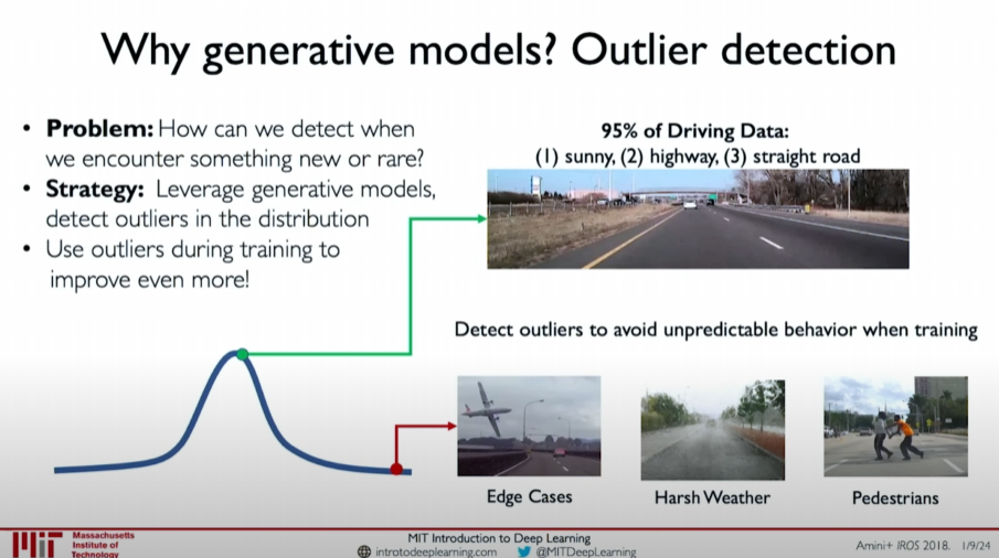
Generative models also play an important role in anomaly detection. In many cases, we need to preemptively detect potential failure modes. For example, in the scenario of autonomous vehicles, certain very rare but critical situations (such as a pedestrian suddenly appearing in front of the car) require the model to be robust enough to handle these cases. By modeling the probability distribution, generative models can automatically detect whether new observations are anomalies, thereby improving model robustness.

Practical Applications of Generative Models

Generative models have important applications in various fields, including:

1. Fairness improvement: By analyzing data distributions, generate fairer training datasets.
2. Anomaly detection: Detect and handle anomalies to improve system robustness.
3. Data augmentation: Generate new data instances to augment training datasets and improve model performance.

Through these applications, generative models demonstrate their potential in building smarter, fairer, and more robust systems.

Latent Variable Models

Course Content Overview

In today’s lecture, we will delve into two types of latent variable models. We will explore the architecture, working principles, and fundamental knowledge and mathematical principles behind these modeling frameworks. Before we start, we need to understand what latent variables are.

Concept of Latent Variables

Latent variables are hidden fundamental elements in data structures that drive the phenomena we measure and observe. To better understand this concept, we can refer to Plato’s “Allegory of the Cave.”

Allegory of the Cave

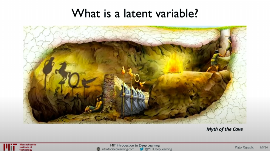
In this allegory, a group of prisoners is forced to stay in a cave, facing one wall of the cave. What they see are only shadows of objects projected on the wall. These shadows are their only perceived reality, but in fact, these shadows are cast by actual objects behind them.

Using this analogy, we can understand that observed variables are like shadows, while latent variables are the actual objects casting the shadows. Latent variables are hidden, underlying factors driving the data we observe.

Goal of Latent Variable Models

The goal of generative models and latent variable models is to learn information about data distributions in an automated way, capturing these underlying driving factors or features. We aim to build a model that represents data distributions and generates new data or understands the features behind the data.

Applications and Architecture of Latent Variable Models

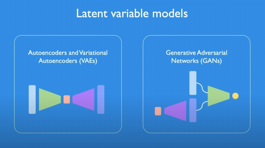
Generative models have broad applications, and the following are two main types of latent variable models:

1. Autoencoder

   • Concept: Autoencoders learn low-dimensional representations of data by compressing and decompressing it.
   • Architecture: Consists of an encoder and a decoder. The encoder compresses high-dimensional data into a low-dimensional latent variable space, and the decoder decodes it back into the original data space.
   • Applications: Dimensionality reduction, feature extraction, denoising, etc.
   • Working Principle:
     1. Data is compressed into a low-dimensional latent variable space by the encoder.
     2. The latent variable is decoded back into the original data space by the decoder.
     3. The model is trained by minimizing the difference between input data and reconstructed data.

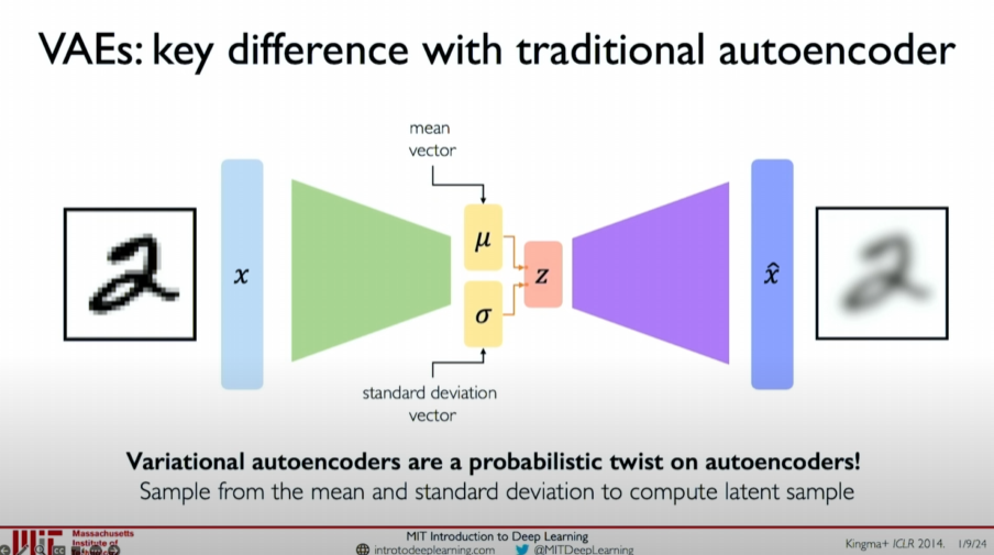
2. Variational Autoencoder (VAE)

   • Concept: VAE introduces the concept of probability distribution to the standard autoencoder, making the generated new data more variable.
   • Architecture: In the latent variable space, VAE learns the mean and standard deviation of latent variables and then samples new data from these distributions.
   • Applications: Image generation, data augmentation, anomaly detection, etc.
   • Working Principle:
     1. The encoder compresses data into the mean and standard deviation of latent variables.
     2. Samples latent variables from these distributions.
     3. The decoder decodes the latent variables into data.
     4. The model is trained by jointly minimizing reconstruction loss and regularization terms.

Importance of Latent Variable Models

Latent variable models provide powerful tools for generating new data and understanding data features by capturing the underlying structure of data. These models are important not only in data compression and feature extraction but also in generating realistic new data, improving model fairness and robustness, and more.

Autoencoders

Course Content Overview

In this section, we will discuss autoencoders in detail. Autoencoders are simple but powerful generative models that learn low-dimensional representations of data for data reconstruction and feature extraction. We will explore their basic concepts, architecture, and training methods.

Basic Concept of Autoencoders

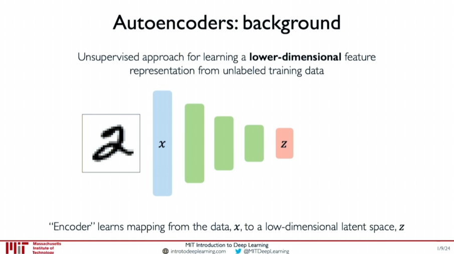
Autoencoders learn effective representations of data

by compressing it into a low-dimensional latent variable space and then decoding it back into the original data space. The core idea is to train the model through an unsupervised learning task, minimizing the difference between input data and reconstructed data.

Example: Image of the Digit “2”

Suppose we have an image of the digit “2”. The autoencoder tries to learn a low-dimensional feature space to faithfully represent this data. The variables in this feature space are called latent variables .

Why Focus on Low Dimensions?

Low-dimensional latent variable spaces have several important advantages:

1. Eliminating Redundancy: Reduces redundant information in the data, improving representation efficiency.
2. Improving Efficiency: Compressing data to lower dimensions allows for more efficient representation of rich data features.

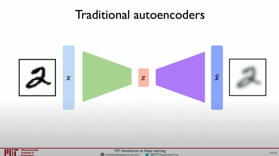
Architecture of Autoencoders

Autoencoders consist of two main parts:

1. Encoder: Compresses the input data into a low-dimensional latent variable space .
2. Decoder: Decodes the low-dimensional latent variable back into the data .

This process can be represented as:

where is the loss function, representing the difference between the original data and the reconstructed data , typically measured using Mean Squared Error (MSE).

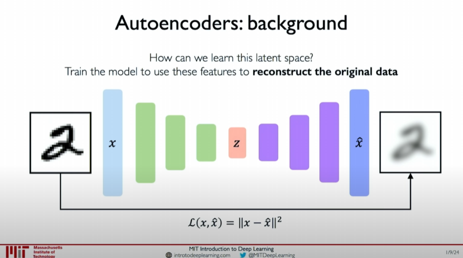
Training Autoencoders

The training of autoencoders is achieved through the following steps:

1. Encoding: Compress the input data into the low-dimensional latent variable space .
2. Decoding: Decode back into the reconstructed data .
3. Minimizing Loss: Compare the input data with the reconstructed data , calculate the reconstruction error (such as Mean Squared Error), and minimize this error.

This process is unsupervised because the model is trained using only the difference between the input data and the reconstructed data, without needing labels.

Applications of Autoencoders

Autoencoders are useful in many applications, such as:

• Dimensionality Reduction: Compress high-dimensional data into lower dimensions for visualization and further analysis.
• Feature Extraction: Extract useful features from raw data for other machine learning tasks.
• Denoising: Remove noise from data to improve data quality.

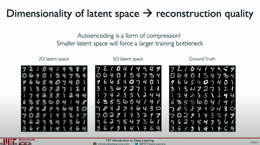
Impact of Latent Space Dimensionality on Reconstruction Quality

An important characteristic of autoencoders is that the dimensionality of the latent space directly affects reconstruction quality. The smaller the latent space dimensionality, the greater the training bottleneck, and the reconstruction quality may be affected. The following images show the impact of different latent space dimensionalities on the reconstruction quality of handwritten digit datasets:

1. 2D Latent Space: Poor reconstruction quality with many details lost.
2. 5D Latent Space: Improved reconstruction quality but still some details are missing.
3. Ground Truth: Original handwritten digit data.

Comparison shows that the larger the latent space dimensionality, the higher the reconstruction quality because a larger latent space can capture and retain more data features.

Core Ideas

1. Data Compression: Autoencoders achieve data reconstruction by compressing data into a low-dimensional latent variable space.
2. Minimizing Reconstruction Error: Train the model by minimizing the error between input data and reconstructed data.
3. Dimensionality Selection: The choice of latent space dimensionality requires a balance between compression efficiency and reconstruction quality.

Autoencoders capture the main features of data by learning a compressed latent variable representation, thereby eliminating redundancy and improving representation efficiency.

Variational Autoencoders (VAEs)

Introduction

Building on the exploration of autoencoders, we now introduce Variational Autoencoders (VAEs). VAEs are more powerful generative models capable of generating new samples. Unlike standard autoencoders, VAEs introduce the concept of randomness and probability distribution, making them more variable when generating new samples.

Limitations of Standard Autoencoders

In standard autoencoders, the representation of latent variables is deterministic. This means that for the same input , the network always generates the same reconstruction . This determinism limits the variability of standard autoencoders in generating new samples.

Introducing Randomness and Probability Distribution

To increase the diversity of generated samples, VAEs achieve this by introducing randomness and actual probability distributions. This approach allows different values to be generated each time for the same input.

Mean and Standard Deviation

In the latent variable layer, VAEs do not directly learn latent variables , but rather learn the mean (mean) and standard deviation (standard deviation) of each latent variable. This way, we can define the probability distribution of each latent variable and sample new data from these distributions.

VAE Architecture

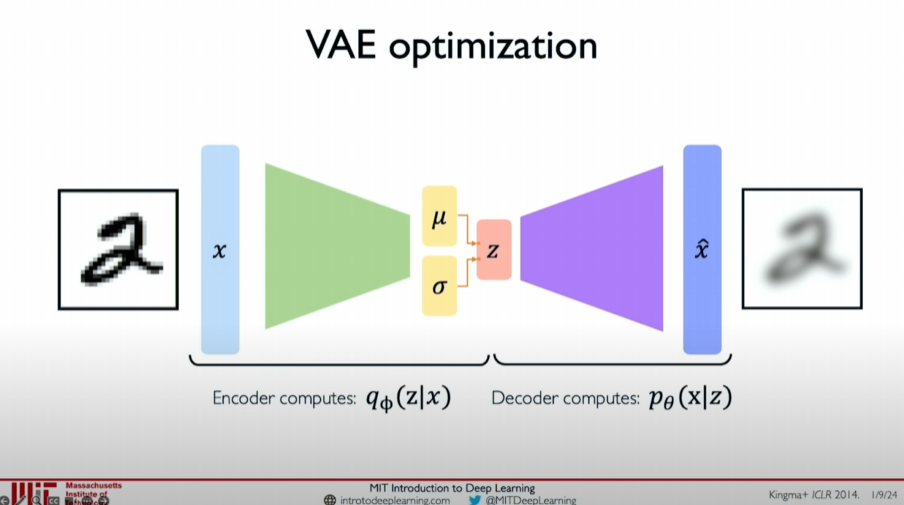
The architecture of VAE can be divided into two stages:

1. Encoder: The encoder calculates the probability distribution of the latent variables given the data , outputting the mean and standard deviation of the latent variables.
   

2. Decoder: The decoder samples new data from the probability distribution of latent variables and decodes it into data .
   

The network weights of the encoder and decoder are represented by and respectively.

Loss Function

The VAE loss function consists of two parts:

1. Reconstruction Loss: Measures the difference between input data and reconstructed data , which can be the log-likelihood or Mean Squared Error (MSE).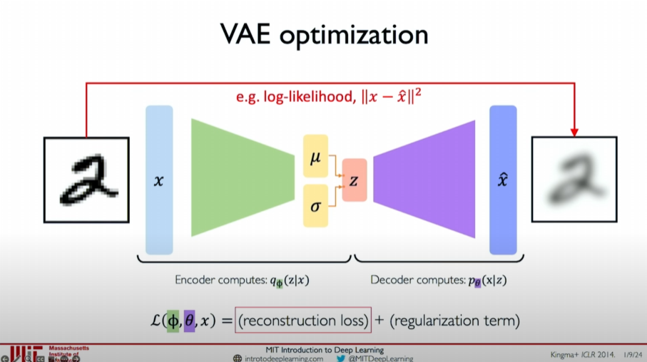

   

2. Regularization Term: Introduces a probability constraint on the latent variable distribution to make the learned latent variable distribution as close as possible to the prior distribution , measured using KL divergence (Kullback-Leibler divergence).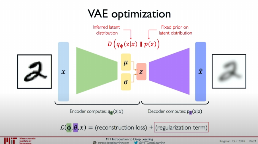

   

The reconstruction loss calculation method is the same as in standard autoencoders and can be expressed using Mean Squared Error (MSE):

The role of the regularization term is to make the learned latent variable distribution as close as possible to the predefined prior distribution (usually a normal distribution). The regularization term can be measured using KL divergence:
$$
\mathcal{L}{\text{KL}} = D{\text{KL}}(q_{\phi}(z|x) | p(z))
$$
where is the learned latent variable distribution and is the prior distribution (usually a standard normal distribution).

The final loss function combines the reconstruction loss and the regularization term:
$$
\mathcal{L}(\phi, \theta, x) = \mathcal{L}{\text{rec}}(x, \hat{x}) + \mathcal{L}{\text{KL}}
$$

Intuitive Understanding

Optimization Process of VAE:

• The encoder calculates the mean and standard deviation of the latent variables.
  

• The decoder samples new data from the probability distribution of latent variables and decodes it into data .
  

• The total loss function combines the reconstruction loss and the regularization term.
  $$
  \mathcal{L}(\phi, \theta, x) = \mathcal{L}{\text{rec}}(x, \hat{x}) + \mathcal{L}{\text{KL}}
  $$

By this method, VAE can not only reconstruct input data but also generate new data instances by sampling. The introduction of the regularization term makes the latent variable distribution more reasonable, ensuring the generated new samples are of high quality and diversity.

I hope this explanation helps you better understand the basic concepts, architecture

, and differences between Variational Autoencoders and standard autoencoders.

Priors on the Latent Distribution

Choice of Prior Distribution

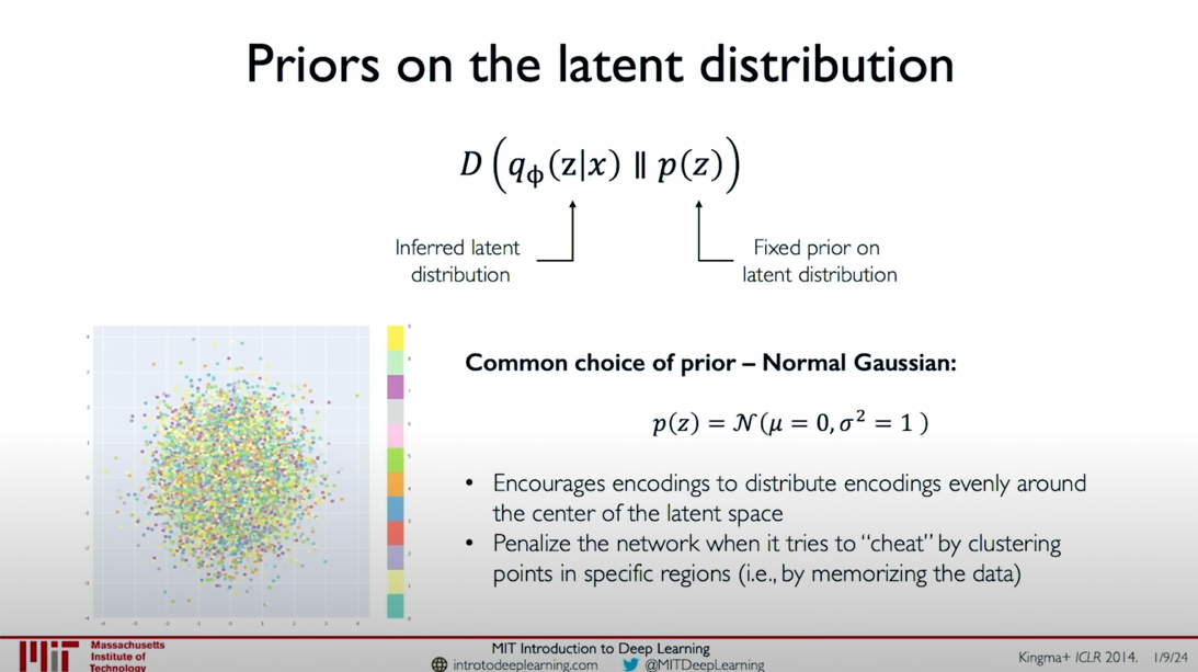
In Variational Autoencoders (VAEs), selecting the prior assumption of the latent variable distribution is a crucial step. The most common approach is to assume that the latent variables follow a normal Gaussian distribution. Specifically, we assume that the mean of each latent variable is 0, and the standard deviation and variance are 1. This normal distribution prior is defined as:

The reasons for choosing a normal distribution as the prior include:

• Uniform Encoding: Encourages the encoding of latent variables to be uniformly distributed around the center of the latent variable space.
• Punishing Clustering: Penalizes the model for clustering points in specific areas to “cheat”, preventing the model from memorizing training data instead of generalizing.

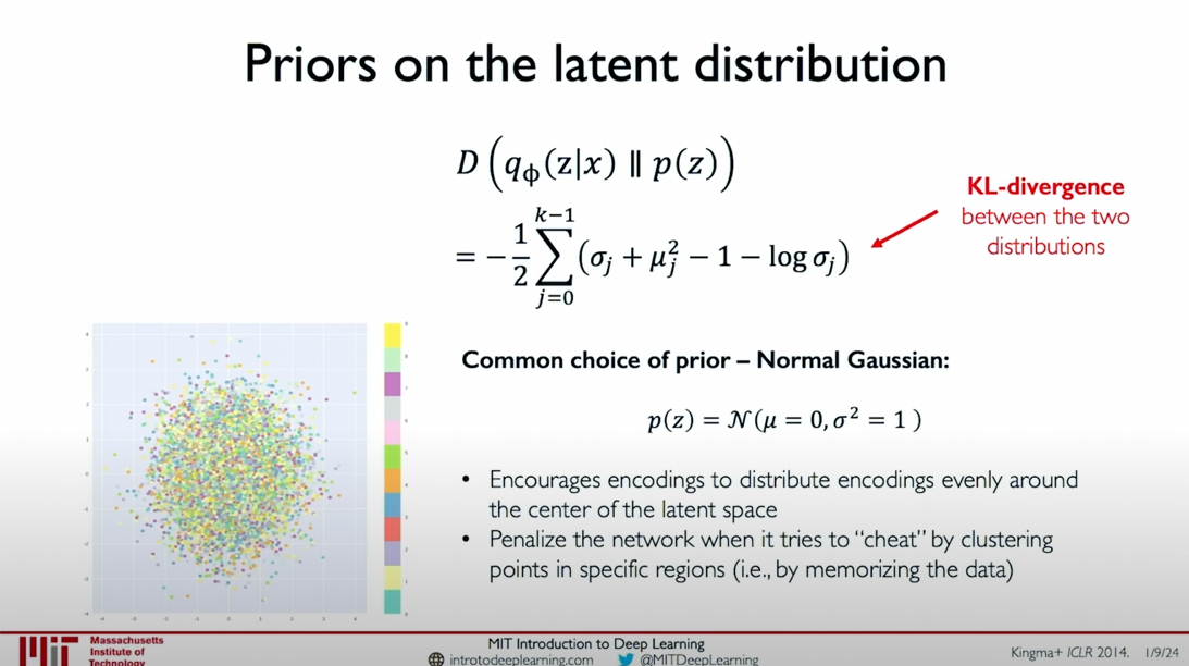
Regularization Term and KL Divergence

To make the learned latent variable distribution as close as possible to the prior distribution , VAE introduces a regularization term. The regularization term is typically measured using KL divergence (Kullback-Leibler divergence):

KL divergence is a distance function that measures the difference between two distributions. For a normal distribution prior, the KL divergence calculation formula is as follows:

where and are the mean and standard deviation of the -th latent variable, respectively.

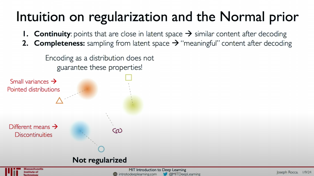
Intuitive Explanation of Regularization and Normal Prior

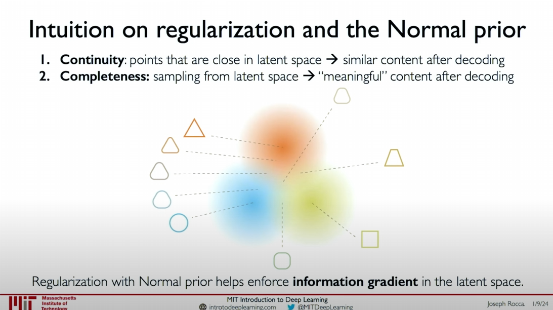
The purpose of introducing regularization and choosing a normal prior is to ensure the continuity and completeness of the latent variable space.

1. Continuity: Points close to each other in the latent variable space should generate similar content when decoded.
2. Completeness: Sampling from the latent variable space should generate meaningful content.

Without regularization, points close to each other in the latent variable space might generate discontinuous content when decoded, resulting in a lack of continuity. For example, two points close to each other in the latent variable space might decode into a square and a triangle, respectively.

With regularization, points close to each other in the latent variable space generate similar and meaningful content when decoded. This ensures that the model generates reasonable samples during the sampling process from the latent variable space.

Specific Examples

1. Without Regularization:

   • Small Variances: Sharp distributions lead to small differences between latent variables.
   • Different Means: Different means lead to different content being generated from points close to each other in the latent variable space.
   • Encoding as distribution does not guarantee continuity and completeness.

   

2. With Regularization:

   • Normal prior ensures centralized means and regularized variances.
   • Continuity: Points close to each other in the latent variable space generate similar content when decoded.
   • Completeness: Sampling from the latent variable space generates meaningful content.
   • With regularization, points close to each other in the latent variable space generate similar and meaningful content when decoded.

   

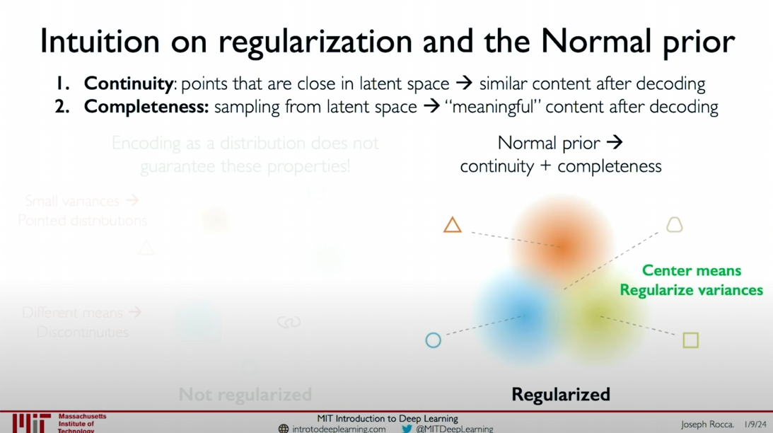
By introducing regularization and choosing a normal prior, VAE can effectively learn the structure of latent variables, generating continuous and meaningful content. These techniques enable VAE to excel in generating high-quality new samples.

I hope this explanation helps you better understand the choice of prior distribution for latent variables, the calculation of the regularization term, and its impact on VAE performance.

Reparameterization Trick

In Variational Autoencoders (VAEs), to effectively perform backpropagation and train the model end-to-end, we use a technique called the Reparameterization Trick.

Core Idea of Reparameterization

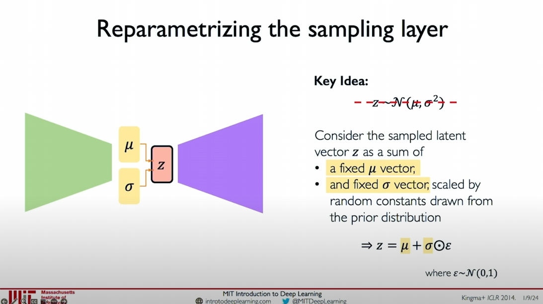
Traditionally, latent variables are directly sampled from a normal distribution , but this makes backpropagation difficult. To overcome this, we introduce the Reparameterization Trick.

The core idea of the Reparameterization Trick is to slightly modify the sampling operation by introducing an additional random variable and reparameterizing the latent variable as follows:

where is the mean vector, is the standard deviation vector, and is a random variable sampled from a standard normal distribution .

This way, we can separate the sampling operation from the latent variable , shifting it to , allowing us to perform backpropagation and optimization on and .

Original Form vs. Reparameterized Form

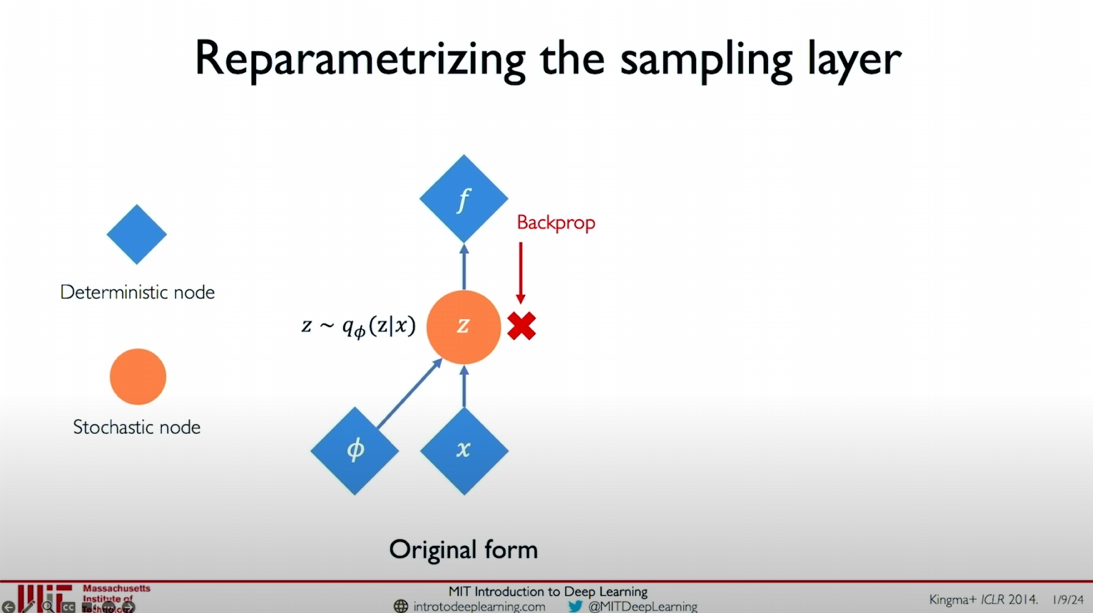
In the original form, the latent variable is directly sampled from the distribution , making it impossible to backpropagate.

Original form:

Why?

In the original form, the latent variable is directly sampled from the distribution , making it impossible to backpropagate. This is because the sampling process introduces non-differentiable randomness.

From a mathematical perspective, suppose we want to optimize the variational lower bound (Variational Lower Bound) through variational inference (Variational Inference), specifically:

$$
\mathcal{L}(\phi, \theta) = \mathbb{E}{q{\phi}(z|x)} \left[ \log p_{\theta}(x|z) \right] - \mathrm{KL}(q_{\phi}(z|x) | p(z)),
$$
where,

• $ \mathbb{E}{q{\phi}(z|x)} \left[ \log p_{\theta}(x|z) \right] z$.
• is the Kullback-Leibler divergence between the latent variable distribution and the prior distribution .

During optimization, we need to compute and update the gradients for the parameters and . However, when is directly sampled from the distribution , this sampling process is inherently discrete and stochastic, making it non-differentiable. This means that gradients cannot propagate through the random variable.

To illustrate this point, consider the expectation in the integral form:

$$
\mathbb{E}{q{\phi}(z|x)} \left[ f(z) \right] = \int f(z) q_{\phi}(z|x) , dz,
$$

where is an arbitrary function of . If we want to compute the gradient with respect to the parameter , we need to solve:

$$
\nabla_{\phi} \mathbb{E}{q{\phi}(z|x)} \left[ f(z) \right] = \nabla_{\phi} \int f(z) q_{\phi}(z|x) , dz.
$$

Since is sampled from the distribution , we need to propagate gradients through the parameters of the distribution . However, the sampling process itself is not continuously differentiable, meaning gradients cannot smoothly propagate through the parameters . This is because the sampling operation lacks continuous differentiability, causing gradient propagation to be obstructed.

To solve this problem, we introduce the Reparameterization Trick. By reparameterizing, we transform the sampling operation into a differentiable function form, allowing gradients to propagate through all variables. Specifically, we introduce a standard normal distribution random variable and express as:

where and are parameters learned from the distribution $q

_{\phi}(z|x)\epsilon\mathcal{N}(0, 1)$.

This way, the sampling process no longer relies on the non-differentiable random variable but instead uses the differentiable variables , , and , allowing us to perform backpropagation and optimization on and .

In summary, the Reparameterization Trick transforms the non-differentiable sampling process into a differentiable function form, enabling us to perform effective backpropagation and optimization, thereby achieving end-to-end training in Variational Autoencoders.

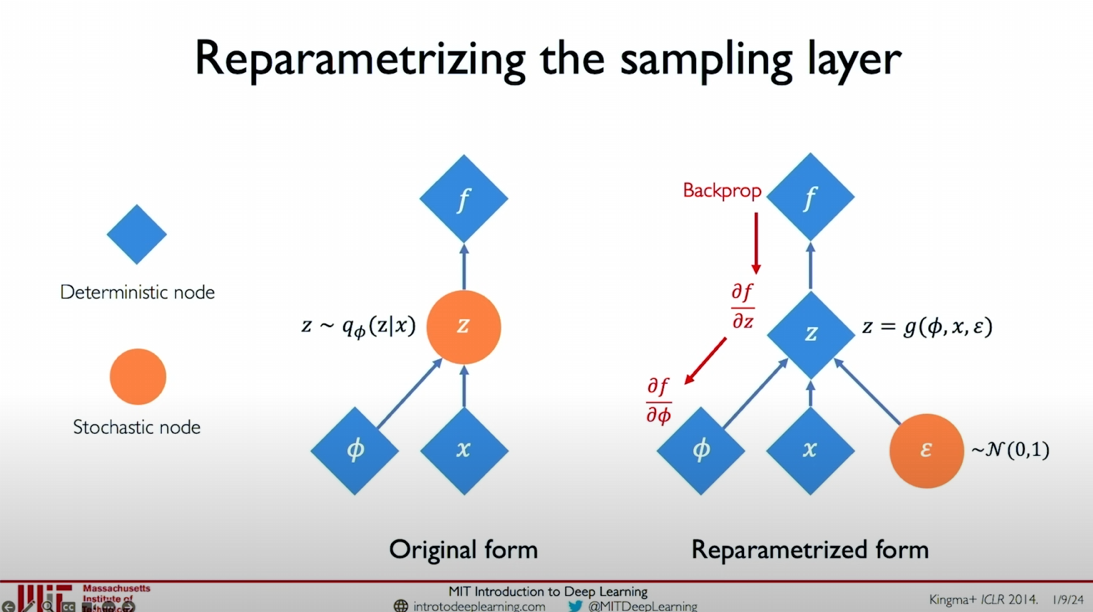
In the reparameterized form, we express as a function of and plus the random variable sampled from the standard normal distribution, allowing us to backpropagate through all variables.

Reparameterized form:

In this form, we can backpropagate through and and compute the corresponding gradients.

The following images compare the structures before and after reparameterization:

1. Original Form: The latent variable is directly sampled from , making it impossible to backpropagate.
2. Reparameterized Form: The latent variable is expressed through , , and the random variable , allowing backpropagation.

By reparameterizing, we can effectively perform backpropagation and train the Variational Autoencoder model end-to-end. This technique is a significant technical breakthrough in VAEs, allowing us to introduce probabilistic and stochastic elements in generative models while retaining backpropagation capabilities.

I hope this explanation helps you better understand the Reparameterization Trick and its role in Variational Autoencoders.

Latent Perturbation and Disentanglement

To understand what the latent variables represent in a trained VAE (Variational Autoencoder) model, we can explore by perturbing a single latent variable while keeping all other latent variables constant, gradually changing the value of that variable, and using the decoder to decode it back into the original data space.

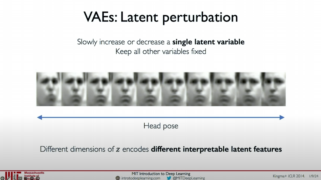
For example, in the illustrated human face example, by perturbing a single latent variable, we can observe the reconstruction of the face changing with the head pose. This indicates that the latent variable captures the head pose and face tilt in the image. This method allows us to explain the role of different dimensions of latent variables in encoding various features.

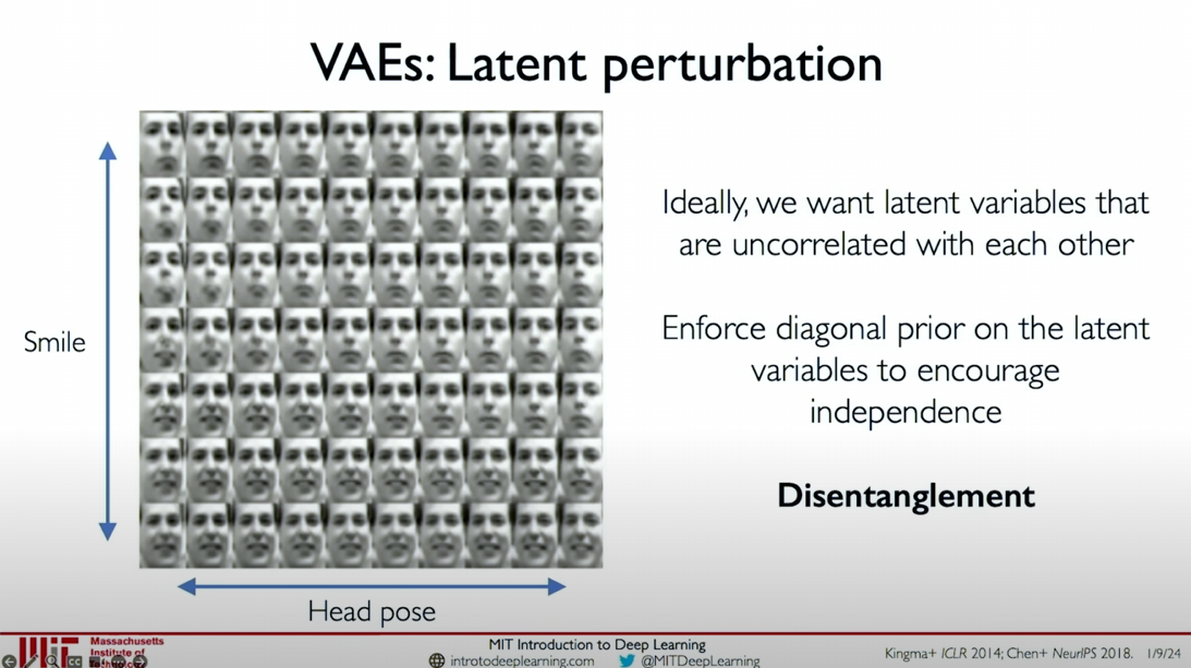
Ideally, we want the latent variables to be as orthogonal as possible, meaning they are independent of each other, as this maximizes the amount of information the model learns in these latent variables. This concept of orthogonality and feature learning is called disentanglement. Disentangling different latent variables (e.g., head pose and smile) is a common goal in training VAE models.

Methods of Disentanglement:

1. Latent Variable Perturbation: Gradually increase or decrease the value of a single latent variable while keeping other variables constant and decode it back into the original data space through the decoder.

   • As shown in the figure, we can see that as the latent variable changes, the head pose in the image changes.

2. Goals of Disentanglement:

   • Continuity: Points close to each other in the latent variable space should decode into similar content.
   • Completeness: Sampling from the latent variable space should generate meaningful content.

3. Implementation of Disentanglement:

   • Regularization Term: Encourage the disentanglement of latent variables by adjusting the relative weights of reconstruction and regularization terms.

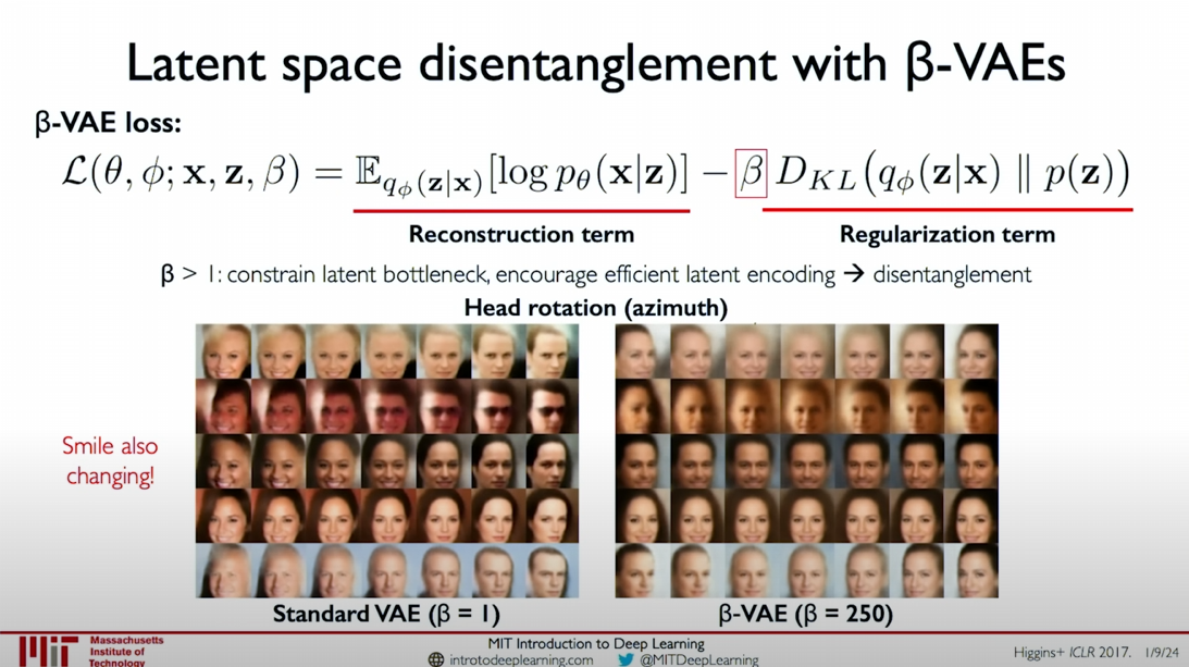
   • β-VAE (Beta-VAE): Adding a weight (β > 1) to the regularization term in the standard VAE can constrain the latent bottleneck, encouraging effective encoding and disentanglement of latent variables.

     • Formula:
       $$
       \mathcal{L}(\theta, \phi; x, z, \beta) = \mathbb{E}{q_\phi(z|x)}[\log p_\theta(x|z)] - \beta D{KL}(q_\phi(z|x) | p(z))
       $$

     • By increasing the weight of the regularization term, latent variables can be better disentangled, making them more interpretable and independent.

The figure shows the disentanglement effects of standard VAE and β-VAE on head rotation and smile. When the regularization term weight is greater than 1 (e.g., β = 250), the model more effectively disentangles the latent variables for head pose and smile.

Summary: By regularizing and adjusting the loss function weights of the model, we can achieve disentanglement of latent variables, making the features in the latent variable space more independent and interpretable. This is important for generating images with different features and understanding the latent features learned by the model.

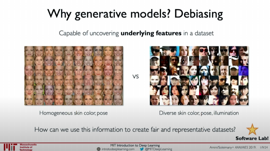
Paper: Uncovering and Mitigating Algorithmic Bias through Learned

Debiasing with VAEs

Why Choose Latent Variable Models? Eliminating Bias

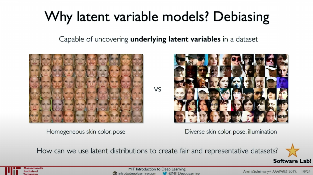
Latent Variable Models can reveal latent variables in datasets, such as skin color, pose, etc. Through these models, we can extract images with diverse skin colors, poses, and lighting conditions from images with homogeneous skin color and pose. This helps create fairer and more representative datasets.

Summary of Variational Autoencoders (VAEs)

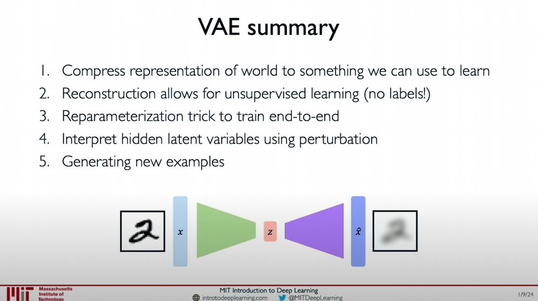
1. Compressed Representation: Compress the representation of the world into something we can use to learn.
2. Reconstruction: Allows unsupervised learning (without labels).
3. Reparameterization Trick: Enables end-to-end training.
4. Interpretation of Latent Variables: Explain latent variables through perturbation analysis.
5. Generate New Samples: Generate new samples.

In practical operations, you will explore and use these models through hands-on experience in a software lab in the context of computer vision and facial detection systems. By explaining and using these features, we can create fairer and more equitable models.

Specific Implementation

The core of Variational Autoencoders is to compress data into a low-dimensional encoding, through which we can generate new samples and understand the features behind the data. This framework allows fully unsupervised reconstruction without the need for data-related labels. We can use the Reparameterization Trick for end-to-end training and explain latent variables through perturbation analysis. Finally, we can sample from the learned latent variables to generate new examples.

Image Analysis

In the image, we can see that on the left is a set of facial images with homogeneous skin color and pose, while on the right is a set of facial images with diverse skin colors, poses, and lighting conditions. This demonstrates the powerful capability of Latent Variable Models in revealing latent variables in datasets, helping us create fairer and more equitable datasets.

I hope this content helps you better understand the basic principles and practical applications of debiasing with VAEs.

Generative Adversarial Networks (GANs)

Theoretical Introduction

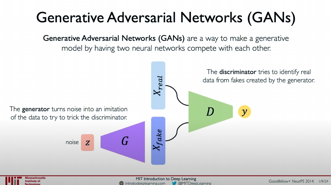
Generative Adversarial Networks (GANs) are a type of generative model that generates data instances through the competition between two neural networks. These two networks are the Generator and the Discriminator.

1. Generator (G):

   • Takes a simple noise vector () as input and generates a fake data instance () through the generator network .
   • The goal of the generator is to generate samples that are as realistic as possible to deceive the discriminator.

2. Discriminator (D):

   • Receives real data instances () and generated data instances () and outputs a probability value indicating the authenticity of the input data.
   • The goal of the discriminator is to distinguish between real data and generated data.

Training Process

The training process of GANs can be seen as a game between the generator and the discriminator:

1. **

Generator Training**:
- The generator samples from a random noise distribution and generates fake data instances.
- The generator updates its parameters by maximizing the probability of the discriminator making incorrect judgments.

2. Discriminator Training:
   • The discriminator updates its parameters by minimizing the probability of incorrect judgments on real data and correct judgments on generated data.

This adversarial process continues until the generator generates data realistic enough that the discriminator cannot distinguish between real and fake data.

Examples and Applications

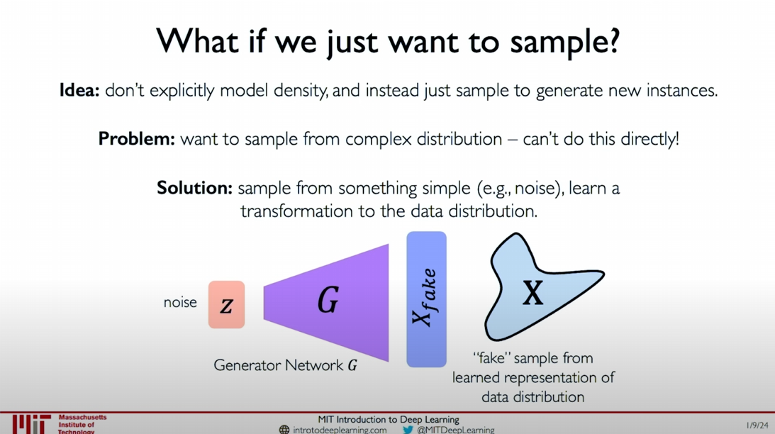
In the illustration, we can see that the generator samples from simple noise (e.g., random noise) and learns to transform this noise distribution into the target data distribution. For example, the generator can learn to transform random noise into the distribution of real images, thereby generating realistic images.

1. Generating New Samples:

   • Generate new data instances (such as images) through the generator, which are visually similar to real data.
   • The generator continuously adjusts to generate increasingly realistic samples until the discriminator cannot distinguish them.

2. Application Scenarios:

   • Image generation: such as generating realistic human face images.
   • Image translation: such as converting a daytime scene image to a nighttime image.

Practical Operation

In the software lab, you will have the opportunity to practice using GANs for image generation. Through experiments, you will gain a deeper understanding of the working principles of Generative Adversarial Networks and learn how to adjust and optimize these networks to generate high-quality samples.

Summary

Generative Adversarial Networks provide a powerful method for generating new data instances, particularly in image generation and translation. Through the competition between the generator and the discriminator, GANs can learn to generate complex and realistic data distributions from simple noise distributions.

I hope this content helps you better understand the basic principles and practical applications of Generative Adversarial Networks. If you have any further questions or need additional explanations, please let me know.

Intuitions Behind GANs

The core idea of Generative Adversarial Networks (GANs) is to generate new data instances through the competition between two neural networks: the Generator and the Discriminator. Here is a detailed explanation and intuitive analysis of this process.

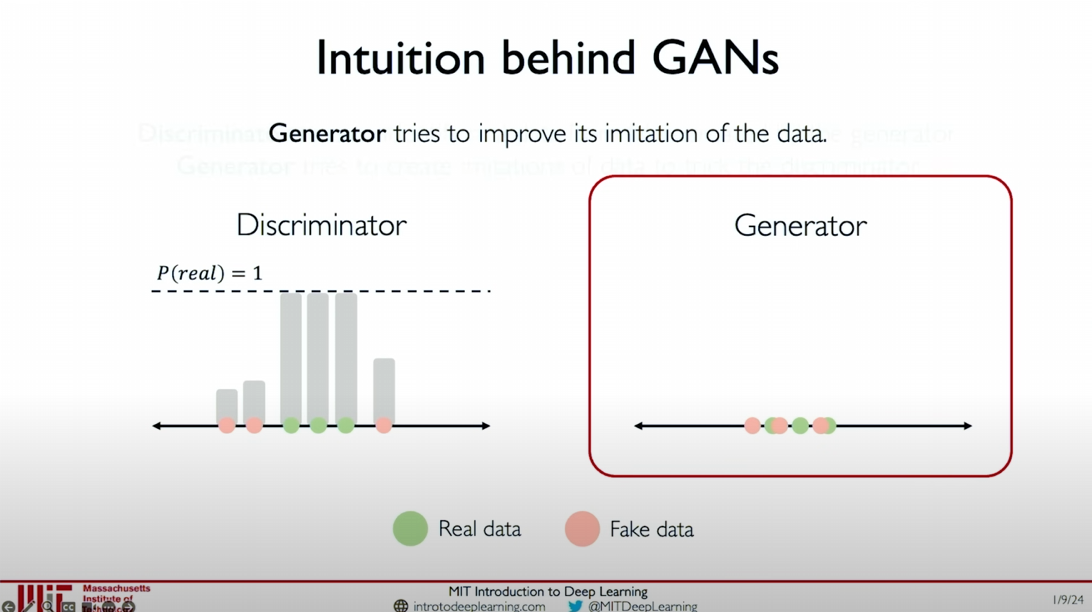
Role of the Generator

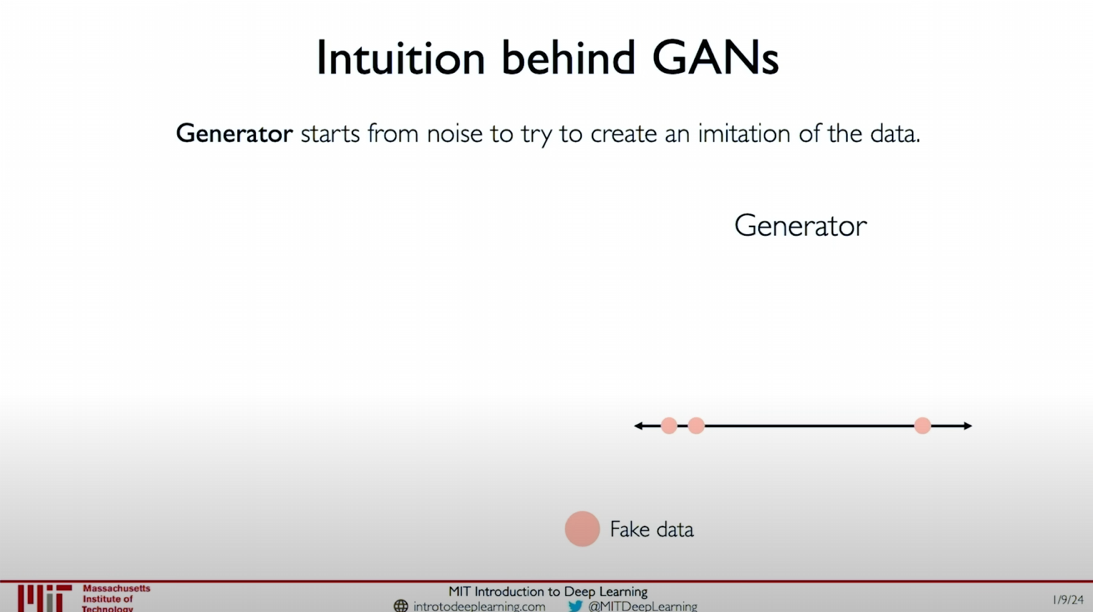
The generator starts from random noise and tries to generate samples that mimic real data.

1. Generate Initial Samples: The generator samples from the noise distribution and generates initial fake data samples (as shown by the orange dots in the figure).
2. Generator’s Goal: The goal of the generator is to generate data samples as realistic as possible to deceive the discriminator.

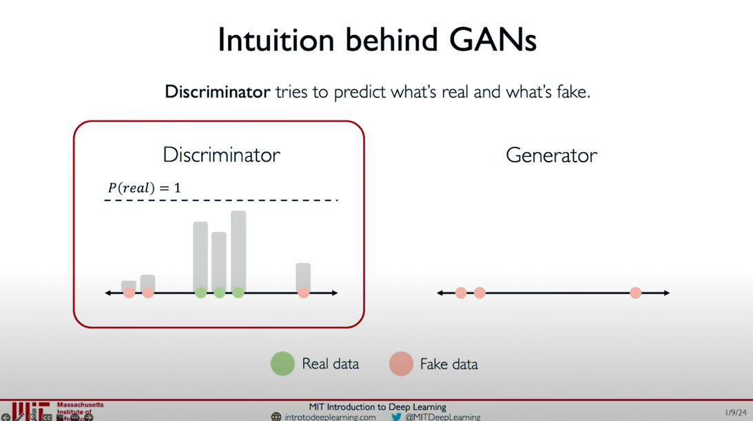
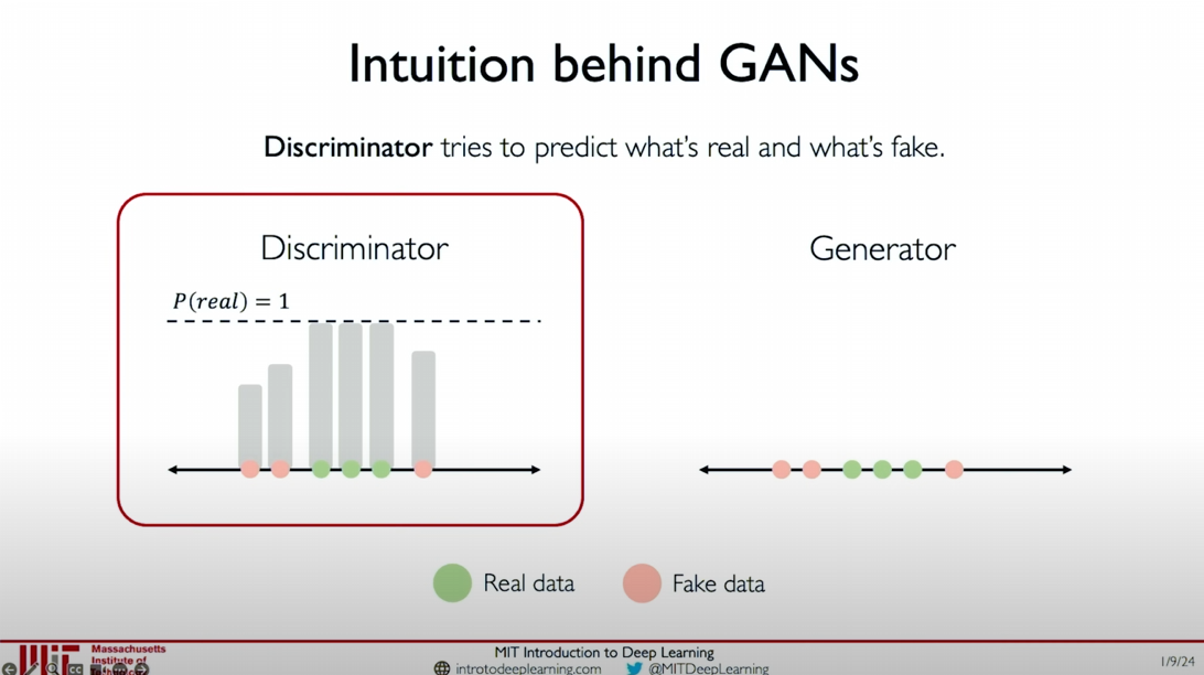
Role of the Discriminator

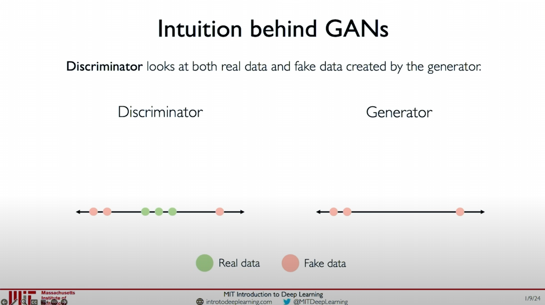
The discriminator’s task is to distinguish between real data and generated data.

1. Training the Discriminator: The discriminator receives real data (green dots) and fake data (orange dots) and outputs the probability for each data point, indicating the likelihood of the data being real.
2. Initial Judgment: In the initial stages, the discriminator’s judgment may not be very accurate, but as training progresses, the discriminator will gradually improve its ability to distinguish between real and fake data.

Adversarial Training Process

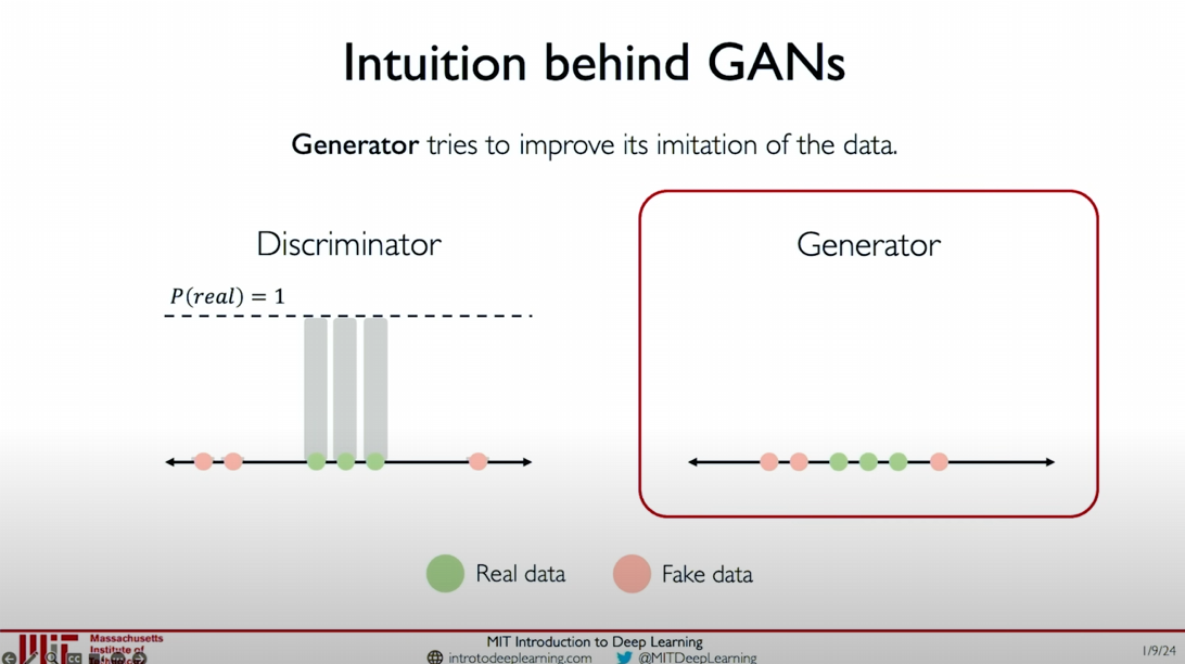
1. Improving the Generator: The generator continuously adjusts its generated data samples based on the feedback from the discriminator to make them more like real data.

   

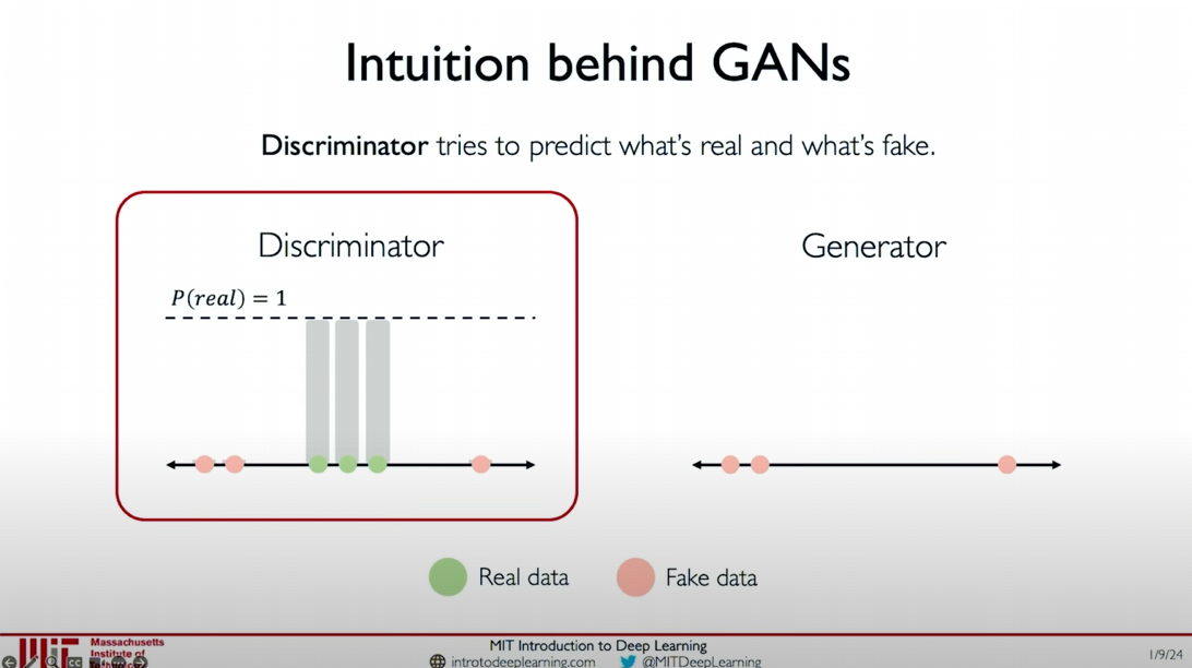
2. Improving the Discriminator: The discriminator continuously receives new real and fake data samples and improves its ability to distinguish between real and fake data by increasing the probability estimate for real data and decreasing the probability estimate for fake data.

   

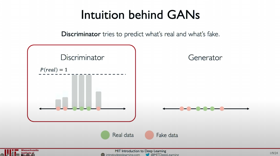
3. Alternating Optimization: This process alternates, with the generator continuously generating more realistic fake data and the discriminator continuously improving its ability to distinguish between real and fake data.

   

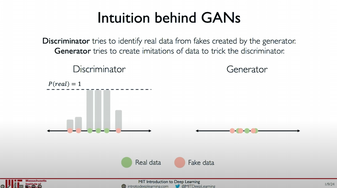
Ultimate Goal

In this adversarial process, both the generator and the discriminator evolve together:

1. Success of the Generator: When the generator generates data samples so realistic that the discriminator cannot distinguish between real and fake data, the generator has successfully learned the target data distribution.
2. Challenge for the Discriminator: The discriminator will continuously try to improve its ability to distinguish between real and fake data, but ideally, the fake data generated by the generator will almost completely overlap with real data, making it difficult for the discriminator to judge.

Intuitive Example

Through the illustrations, we can see:

1. Initial Stage: The fake data samples generated by the generator (orange dots) are far from the real data samples (green dots).
2. Intermediate Stage: As training progresses, the fake data samples generated by the generator gradually approach the real data distribution, making it increasingly difficult for the discriminator to distinguish.
3. Final Stage: The fake data samples almost completely overlap with the real data samples, making it difficult for the discriminator to distinguish between real and fake data, indicating that the generator has achieved its goal.

This adversarial mechanism allows GANs to excel in image generation, data augmentation, and other fields. By continuously improving, the generator can generate highly realistic data samples.

Summary

Through the adversarial training of the generator and the discriminator, GANs can generate realistic data samples from simple random noise. The key in this process is how the generator continuously improves its generated samples to approach real data, while the discriminator continuously enhances its judgment ability, ultimately achieving the effect that the generator generates data indistinguishable from real data.

I hope this content helps you better understand the intuitions and working principles of GANs.

Training GANs

Framework Concept Summary

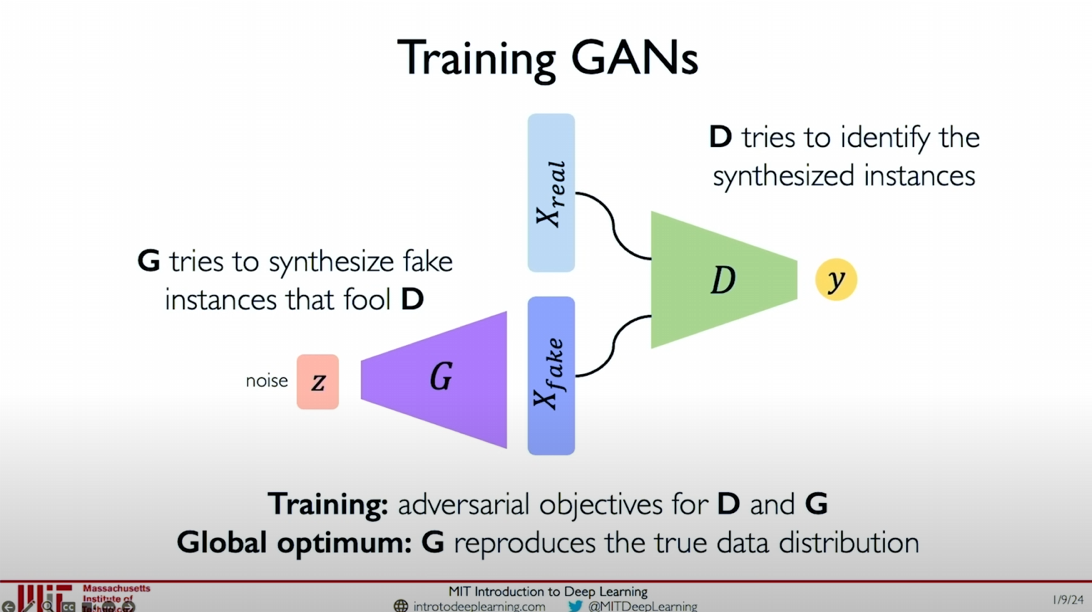
The basic framework of Generative Adversarial Networks (GANs) contains two core components: the Generator and the Discriminator. The generator tries to synthesize fake data instances to deceive the discriminator, while the discriminator tries to distinguish between real and fake instances. During training, the goal of GANs is to achieve the competing objectives of the generator and the discriminator through the loss function.

1. Generator (G):

   • The goal of the generator is to generate data samples as realistic as possible so that the discriminator cannot distinguish between real and fake.
   • Synthesizes fake data instances to deceive the discriminator.

2. Discriminator (D):

   • The goal of the discriminator is to accurately distinguish between real data and generated data.
   • Learns from real data and generated data and tries to identify synthesized fake instances.

Training Objectives

The training objective of GANs is to make the generator perfectly reproduce the real data distribution while the discriminator cannot distinguish between real and fake data at all. In practice, this optimal situation is very difficult to achieve. Training GANs is challenging and often encounters mode collapse and unstable training issues.

Stable Training Techniques

To improve the stability of GANs training, researchers have proposed various improvement methods, including modifying the loss function and using stable training techniques. Nevertheless, training GANs remains a challenging process.

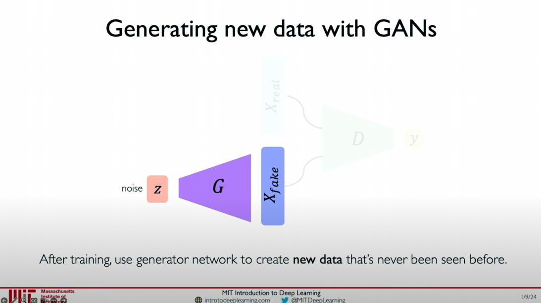
Using GANs

Once the GAN model is successfully trained, we can generate new data instances through the generator. The specific steps are as follows:

1. Back to the Generator:

   • Starting from random noise , generate new data instances through the generator .

2. Generate New Data:

   • Select different points from the initial distribution of random noise and generate new data instances through the generator.

Distribution Transformation

![image-20240609213512694](https://cdn.jsdelivr.net/gh/xiwuqi/image-hosting

@master/picgo/202406092135854.png)

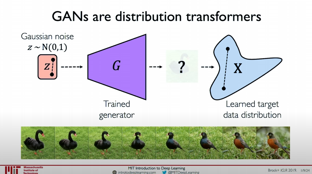
GANs essentially act as distribution transformers, learning to transform Gaussian noise distribution into the target data distribution. The specific steps are:

1. Initial Noise: Sample from Gaussian noise .
2. Generator Learning: The generator learns to transform the noise distribution into the target data distribution .
3. Target Distribution: The generated samples approach the target data distribution, and the generator successfully achieves the transformation from noise to data.

Traversal and Interpolation

By learning the distribution transformation, we can traverse and interpolate in the Gaussian noise space to generate different samples. The generator can transform these noise samples into samples in the target data distribution, achieving diversity in generated data.

Generate Similar Images

By applying the same type of initial perturbation, we can generate progressively similar images in the target distribution. For example, starting from noise samples, progressively generate visually similar images.

Summary

GANs are a very concise and powerful framework that can generate realistic data samples from simple random noise through the adversarial training of the generator and the discriminator. Although the training process is challenging, GANs have broad application prospects in image generation, data augmentation, and other fields. I hope this content helps you better understand the training process and practical applications of GANs. If you have any further questions or need additional explanations, please let me know.

GANs: Recent Advances

Basic Framework of GANs

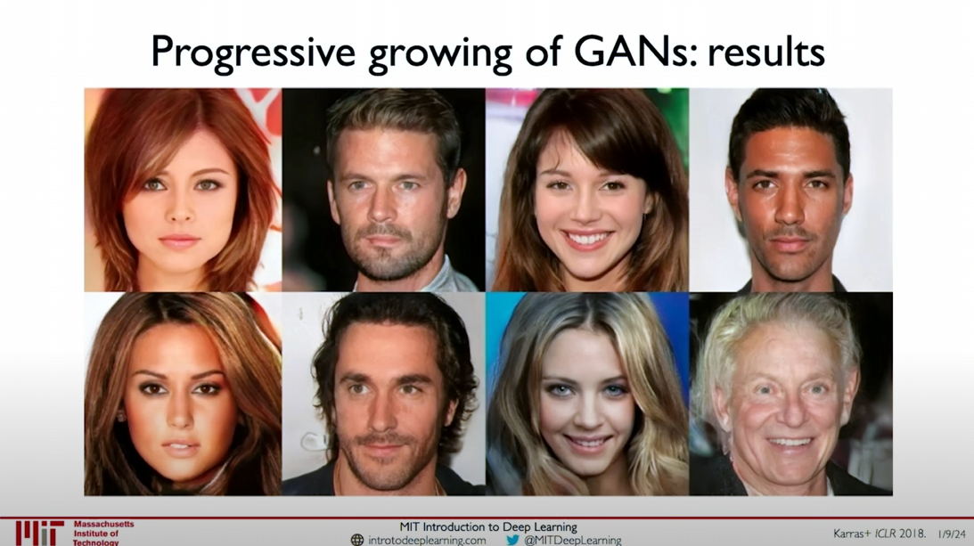
Generative Adversarial Networks (GANs) are a very concise and powerful framework for generating realistic data samples. For example, the architecture of GANs is used to generate facial images, as we saw in the previous slides. In recent years, researchers have proposed various improvement methods to enhance the effectiveness of GANs from a modeling perspective.

Conditional GANs

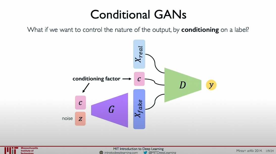
An important advancement is Conditional GANs, which allow better control over the generation process. By adding different types of conditional information, we can guide the generator to generate samples that meet specific conditions. For example, instead of using random noise as the starting point, we can also consider other forms of conditional factors that can guide the generation process.

Paired Translation

A core idea is the concept of paired translation, which means we can use paired inputs for training. For example, a scene and its corresponding segmentation map. We can train the discriminator to operate not only on single inputs but on paired inputs, judging the authenticity of pairs of images and segmentation maps.

This way, the generator can accept an input of a segmented scene and generate an output of a real-world view scene, or convert a street map to a grid view, and so on. This paired translation method is widely applied to various image translation tasks, such as converting map views to aerial views or vice versa.

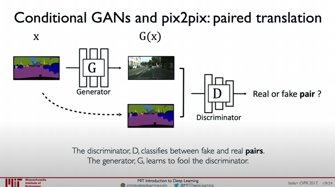
Conditional GANs and pix2pix

A practical application of Conditional GANs is the pix2pix framework, which is used for paired translation tasks. In pix2pix, the generator is responsible for converting the input image into the target image , while the discriminator is used to distinguish between real and generated image pairs.

1. Generator :

   • Accepts the input image and generates the target image .

2. Discriminator :

   • Distinguishes between real image pairs and generated image pairs.

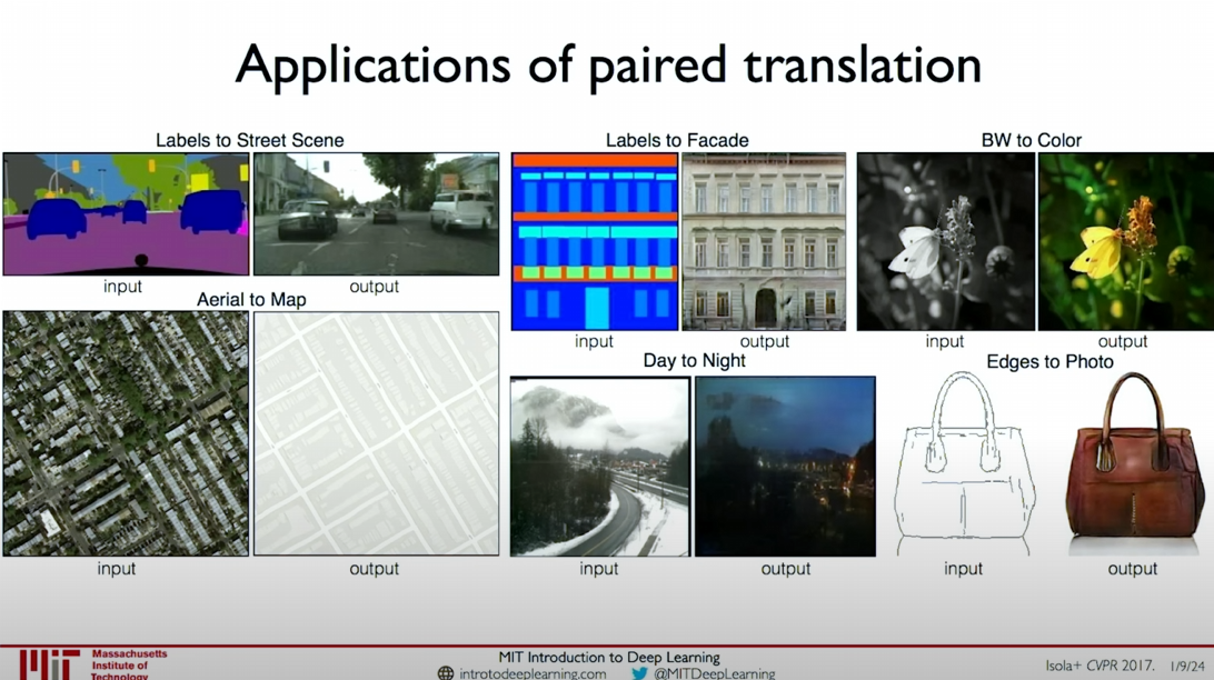
This method allows us to apply to different image translation tasks, such as:

• Labels to Street Scene
• Labels to Facade
• BW to Color
• Aerial to Map
• Day to Night
• Edges to Photo

Results of Paired Translation

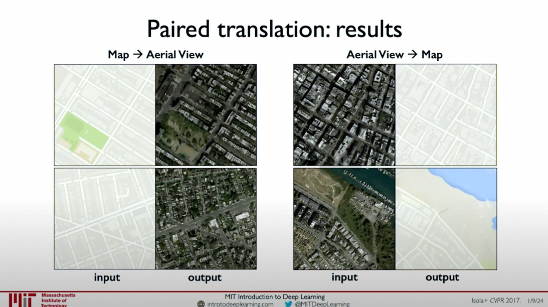
Through Paired Translation, GANs can achieve conversions from map views to aerial views, and vice versa. The following are practical application examples:

• Map to Aerial View:

  • Input: Map view
  • Output: Aerial view

• Aerial View to Map:

  • Input: Aerial view
  • Output: Map view

Summary

GANs are a very flexible and powerful tool, and with continuous development and improvement, we can achieve increasingly complex and precise generation tasks. Conditional GANs and paired translation methods allow us to add more control conditions in the generation process, thereby generating samples that better meet expectations. These advancements not only expand the application range of GANs but also provide new possibilities for various image generation and translation tasks.

I hope this content helps you better understand the latest advancements and practical applications of GANs.

CycleGAN of Unpaired Translation

In the previous explanations, we learned about the basic concepts of Generative Adversarial Networks (GANs) and how they generate realistic data instances through the adversarial training of the generator and the discriminator. GANs primarily achieve data distribution transformation from Gaussian Noise to Target Data Distribution.

In the further development of GANs, CycleGAN emerged to solve the problem of domain translation without paired data. The core concept of CycleGAN is to learn data distribution transformation between two different domains through cyclic consistency loss.

Basic Architecture

CycleGAN consists of two generators and two discriminators:

• Generator G: Responsible for transforming data from domain X to domain Y (i.e., G: X -> Y).
• Generator F: Responsible for transforming data from domain Y to domain X (i.e., F: Y -> X).
• Discriminator Dx: Responsible for distinguishing real data from domain X and fake data generated by generator F.
• Discriminator Dy: Responsible for distinguishing real data from domain Y and fake data generated by generator G.

Loss Function

The training of CycleGAN relies on two main loss functions:

• Adversarial Loss: Used to train the generators and discriminators to make the generated images as realistic as possible.
  • Adversarial loss of generator G: The goal is to make the images generated by generator G as similar as possible to real images from domain Y to deceive discriminator Dy.
  • Adversarial loss of generator F: The goal is to make the images generated by generator F as similar as possible to real images from domain X to deceive discriminator Dx.
• Cyclic Consistency Loss: Ensures that after transforming through both generators, the original image can be recovered.
  • Loss from domain X to domain Y and back to domain X (X -> G(X) -> F(G(X)) -> X).
  • Loss from domain Y to domain X and back to domain Y (Y -> F(Y) -> G(F(Y)) -> Y).

Training Process

• Train generators G and F to generate images that can deceive the corresponding discriminators.
• Train discriminators Dx and Dy to correctly distinguish between real and generated images.
• Optimize the parameters of the generators and discriminators by minimizing the adversarial loss and cyclic consistency loss.

1. Basic Principles of CycleGAN

   

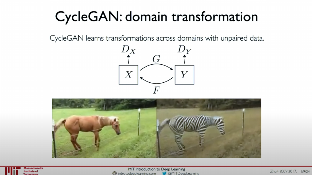
   • Suppose we have two different data domains X and Y without direct pairing relationships. CycleGAN learns the mapping from domain X to domain Y (G) and the inverse mapping from domain Y to domain X (F) to achieve data translation between the two domains.
   • The key to this translation is to ensure that the result after transforming from X to Y through G and then back to X through F should be as consistent as possible with the original X, and vice versa. This is the so-called cyclic consistency loss.

2. Application Examples

   • Horse and Zebra Translation: In the classic example of CycleGAN, we can see that images of horses are translated into images of zebras and vice versa. This translation involves not just color and texture changes but also changes in the background grass color, demonstrating CycleGAN’s ability to translate the entire image distribution.

   • Voice Translation: CycleGAN can also be used for voice domain translation. By converting audio waveforms into spectrogram images and performing translation between different spectrograms, CycleGAN can achieve voice translation between different speakers. For example, converting Alexander’s voice to Obama’s voice.

     

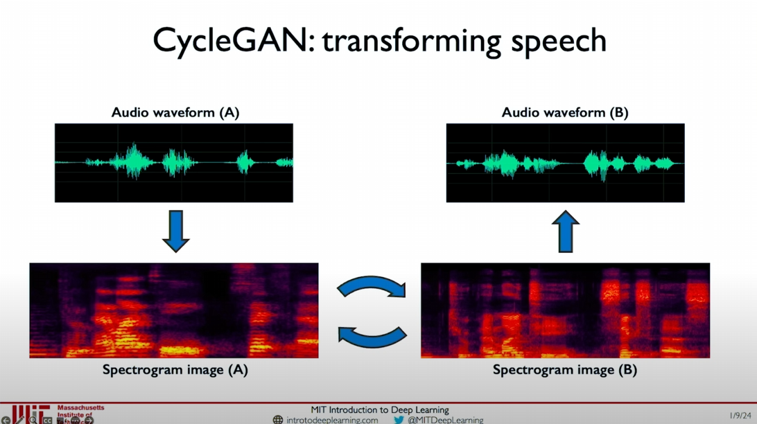
     In this example, we convert the speech waveform to a spectrogram and use CycleGAN for domain translation. For instance, we record Alexander’s voice and convert it to a spectrogram, and also record Obama’s voice and convert it to a spectrogram. By training CycleGAN, we can achieve translation between Alexander’s voice and Obama’s voice.

3. Implementation Details

   

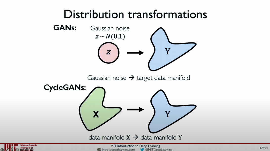
   • Distribution Transformation: A significant function of CycleGAN is its ability to perform data distribution transformation without paired data. Traditional GANs achieve transformation from Gaussian noise to the target data manifold, while CycleGAN achieves transformation

between two data manifolds.

Through CycleGAN, we can achieve data domain translation without paired data, significantly expanding the application scope and practicality of Generative Adversarial Networks. CycleGAN has demonstrated powerful capabilities in image translation, voice translation, and more, making it an important tool in generative modeling.

We have discussed two types of deep generative models: Autoencoders and Variational Autoencoders (VAEs), and Generative Adversarial Networks (GANs). The former learns low-dimensional representations and encodings of data, while the latter generates new data instances through adversarial networks. CycleGAN is a specific type of GAN that achieves domain translation without paired data through cyclic consistency loss.

The introduction of CycleGAN has significantly advanced generative modeling and generative AI, with applications extending beyond image and voice translation to more fields.

Summary:
By introducing cyclic consistency loss, CycleGAN solves the problem of domain translation without paired data, allowing us to achieve high-quality translation between different data distributions. This method has broad application prospects in image and voice translation, further promoting the development and application of Generative Adversarial Networks.

Diffusion Model Sneak Peek

Diffusion models are a type of generative model conceptually very close to Variational Autoencoders (VAEs). They perform exceptionally well in generating new instances, particularly with very high fidelity. Additionally, diffusion models can be guided and adjusted based on different forms of input, such as text or other types of modalities.

As seen in the image, diffusion models generate highly realistic images. These models excel not only in image generation but also have broad applications in other fields. Tomorrow’s lecture will delve into the working principles of these models and their applications in various fields.

Course Summary

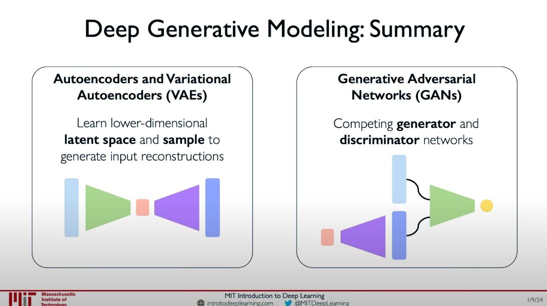
In this course, we primarily explored two major types of deep generative models:

1. Autoencoders and Variational Autoencoders (VAEs):

   • Learn low-dimensional latent spaces and sample from them to generate input reconstructions.
   • Compress input data into the latent space through the encoder and restore data from the latent space through the decoder.

2. Generative Adversarial Networks (GANs):

   • Consist of an adversarial network of a generator and a discriminator.
   • The generator tries to generate realistic fake data to deceive the discriminator, while the discriminator tries to distinguish between real and fake data.
   • Through adversarial training, the generator can eventually generate highly realistic data.

3. Diffusion Models:

   • Similar to VAEs, diffusion models have very high fidelity when generating new instances.
   • Can be guided and adjusted based on different forms of input to achieve higher control over the generation process.

Extended Content

To better understand these models, we also discussed various GANs variants and advanced applications, including:

• Conditional GANs: Control the nature of generated data by adding conditional inputs.
• CycleGAN: Achieve domain translation without paired data.
• Recent Advances: Explored the latest applications of GANs in image generation, audio translation, etc.

Post-Lecture Experiment

http://introtodeeplearning.com#schedule
https://github.com/aamini/introtodeeplearning/

Closing Remarks

Through this course, you should have a comprehensive understanding of deep generative models, including their principles, implementation methods, and application scenarios. I hope this knowledge helps you conduct relevant research and projects in computer vision, natural language processing, and other fields.

Thank you all for your participation and learning. See you in the next class!

---

---

---

CN

Introduction

Introduction: 生成建模简介

图中三个人都是生成的，没有一个是真人

课程概述

在这个讲座中，我们将讨论生成模型（Generative Model）或生成式人工智能（Generative AI）的概念。近年来，生成式人工智能成为热门话题，引起了广泛关注和讨论。在本次讲座中，我们将深入了解生成建模的基础，探索其核心思想：构建能够不仅识别数据模式并做出决策，还能基于所学模式生成全新数据实例的系统。

生成建模的定义

生成建模的核心是构建一种能够模拟数据分布并生成新数据的系统。生成模型不仅限于传统的监督学习（Supervised Learning），其重点在于无监督学习（Unsupervised Learning）。在无监督学习中，我们的目标不是学习从输入 到输出 的映射，而是分析输入数据 本身，学习其潜在模式和特征。

监督学习 vs. 无监督学习

1. 监督学习（Supervised Learning）
   • 有标签数据：每个实例都附有一个标签。
   • 目标：学习输入数据与标签之间的映射关系。
   • 应用：分类（Classification）、回归（Regression）、分割（Segmentation）等。
2. 无监督学习（Unsupervised Learning）
   • 无标签数据：仅有输入数据，无明确标签。
   • 目标：学习数据的潜在结构和模式。
   • 应用：密度估计（Density Estimation）、聚类（Clustering）等。

生成模型的实现

生成模型主要通过两种方式实现：

1. 密度估计（Density Estimation）

   • 学习并拟合数据的概率分布。
   • 目标：找到一个模型来模拟数据的概率分布。

2. 样本生成（Sample Generation）

   • 从学习到的概率分布中抽取新样本。
   • 目标：利用已学的概率分布生成新的数据实例。

生成建模的这两个用例的共同点是我们如何训练一个非常好的概率分布模型，该模型类似于我们真实数据的真实概率分布

生成建模的应用

生成模型具有广泛的应用，不仅限于生成逼真的人脸图像。其在多种领域中都有重要作用，例如：

• 图像生成（Image Generation）
• 文本生成（Text Generation）
• 音乐生成（Music Generation）

课程实例：生成假人脸

在本讲座中，我们将探讨如何通过生成模型（例如StyleGAN）生成逼真的人脸图像。StyleGAN是一种生成对抗网络（GAN），能够生成高质量、逼真的图像。通过这些实例，我们将深入了解生成模型的工作原理及其实现方法。

结论

生成建模是一种强大的技术框架，其核心在于学习并模拟数据的概率分布。通过生成建模，我们不仅可以识别数据模式，还可以生成新数据，从而在各种应用中展示其强大功能。在接下来的课程中，我们将进一步探讨生成模型的具体实现技术和应用场景。

希望通过这部分讲解，你对生成建模有了一个初步的认识，并对接下来的学习充满期待。

Why Care About Generative Models?

生成模型的重要性

生成模型（Generative Models）不仅仅是为了生成新的数据实例，它们在多个方面具有重要的应用和意义。这部分讲解将涵盖生成模型在公平性、异常检测等领域的应用，并解释这些模型为什么如此重要。

智能学习与公平性

生成模型能够利用概率分布的信息来进行更智能的学习。通过分析哪些数据特征在总体分布中更具代表性，可以训练出在不同数据特征上的表现更公平、偏差更小的模型。这种方法有助于：

• 提高模型的公平性：使用生成模型生成更具代表性的数据集，减少数据中的偏差，进而训练出更公平的模型。
• 减少偏差：通过理解数据分布，可以识别并减少模型在特定数据特征上的偏差。

在课程的第二个实验中，你将亲自体验如何利用这些学习到的特征来创建更公平的数据集和模型。

异常检测

生成模型在异常检测（Outlier Detection）中也发挥着重要作用。许多情况下，我们需要预先检测可能的故障模式。例如，在自动驾驶汽车的场景中，某些非常罕见但至关重要的情况（如行人突然出现在车前）需要模型具备鲁棒性来处理这些情况。生成模型通过建模概率分布，能够自动检测新的观察结果是否属于异常，进而改进模型的鲁棒性。

生成模型的实际应用

生成模型在多个领域都有重要应用，以下是几个主要的应用场景：

1. 公平性改进：通过分析数据分布，生成更公平的训练数据集。
2. 异常检测：检测和处理异常情况，提高系统的鲁棒性。
3. 数据增强：生成新的数据实例来增强训练数据集，提高模型性能。

通过这些应用，生成模型展示了其在构建更智能、更公平和更鲁棒系统中的潜力。

Latent variable models

课程内容概述

在今天的讲座中，我们将深入研究两类潜变量模型（Latent Variable Models）。我们将探讨这些模型的架构、工作原理，并传达这些建模框架背后的基础知识和数学原理。在开始之前，我们首先需要了解什么是潜变量。

潜变量的概念

潜变量（Latent Variables）是数据结构中隐藏的基本元素，它们驱动我们所测量和观察到的现象。为了更好地理解这一概念，我们可以参考柏拉图的“洞穴神话”。

洞穴神话

在这个神话中，有一群囚犯被迫待在一个洞穴里，只能面对洞穴的某一面墙。他们所看到的只是投射在墙上的物体的影子。这些影子是他们唯一能观察到的现实，但实际上，这些影子是由他们背后实际存在的物体投射的。

通过这个类比，我们可以理解，观察到的变量（Observed Variables）就像影子，而潜变量则是那些实际存在并投射影子的物体。潜变量是隐藏的、底层的因素，驱动着我们观察到的数据。

潜变量模型的目标

生成模型和潜变量模型的目标是通过自动化的方法，学习关于数据分布的信息，捕获这些潜在的驱动因素或特征。我们希望构建一个能够表示数据分布的模型，进而生成新数据或理解数据背后的特征。

潜变量模型的应用与架构

生成模型的应用广泛，以下是两类主要的潜变量模型：

1. 自动编码器（Autoencoder）

   • 概念：自动编码器通过压缩和解压数据来学习数据的低维表示。
   • 架构：包括编码器和解码器两部分。编码器将高维数据压缩到低维潜变量空间，解码器则将其解码回原始数据空间。
   • 应用：数据降维、特征提取、去噪等。
   • 工作原理：
     1. 数据经过编码器，被压缩到低维潜变量空间。
     2. 潜变量通过解码器被还原到原始数据空间。
     3. 通过最小化输入数据与重建数据之间的差异来训练模型。

2. 变分自动编码器（Variational Autoencoder, VAE）

   • 概念：VAE在标准自动编码器的基础上，引入概率分布的概念，使得生成的新数据具有更多的变异性。
   • 架构：在潜变量空间中，VAE学习潜变量的均值和标准差，然后从这些分布中采样生成新数据。
   • 应用：图像生成、数据增强、异常检测等。
   • 工作原理：
     1. 编码器将数据压缩到潜变量的均值和标准差。
     2. 从这些分布中采样得到潜变量。
     3. 解码器将潜变量解码为数据。
     4. 通过重建损失和正则化项共同训练模型。

潜变量模型的重要性

潜变量模型通过捕捉数据的底层结构，提供了生成新数据和理解数据特征的强大工具。这些模型不仅在数据压缩和特征提取中发挥重要作用，还在生成逼真的新数据、提高模型的公平性和鲁棒性等方面展示了巨大的潜力。

Autoencoders

课程内容概述

在本节中，我们将详细讲解自动编码器（Autoencoder）。自动编码器是一种简单但功能强大的生成模型，它通过学习数据的低维表示来实现数据重建和特征提取。我们将探讨其基本概念、架构和训练方法。

自动编码器的基本概念

自动编码器通过将数据压缩到低维潜变量空间，然后再解码回原始数据空间来学习数据的有效表示。其核心思想是通过无监督学习任务来训练模型，最小化输入数据和重建数据之间的差异。

示例：数字“2”的图像

假设我们有一个包含数字“2”的图像，自动编码器会尝试学习一个低维特征空间，以忠实地表示这个数据。这个特征空间中的变量我们称之为潜变量 ​。

为什么关注低维度？

低维度的潜变量空间有几个重要优点：

1. 消除冗余：减少数据中的冗余信息，提高表示的效率。
2. 提高效率：压缩数据到较低维度，从而更有效地表示数据的丰富特征。

自动编码器的架构

自动编码器由两个主要部分组成：

1. 编码器（Encoder）：将输入数据 压缩到低维潜变量空间 。
2. 解码器（Decoder）：从低维潜变量 解码并重建数据 。

这个过程可以表示为：

其中， 是损失函数，表示原始数据 与重建数据 之间的差异，通常使用均方误差（Mean Squared Error, MSE）来衡量。

训练自动编码器

自动编码器的训练通过以下步骤实现：

1. 压缩（Encoding）：将输入数据 压缩到低维潜变量空间 。
2. 解码（Decoding）：将 解码回重建数据 。
3. 最小化损失（Minimize Loss）：通过比较输入数据 和重建数据 ，计算重建误差（例如均方误差），并最小化这个误差。

这个过程是无监督的，因为我们只需使用输入数据和重建数据之间的差异来训练模型，而不需要标签。

自动编码器的应用

自动编码器在许多应用中都非常有用，例如：

• 数据降维：将高维数据压缩到低维空间，便于可视化和进一步分析。
• 特征提取：从原始数据中提取有用的特征，用于其他机器学习任务。
• 去噪（Denoising）：去除数据中的噪声，从而提高数据质量。

潜变量空间的维度对重建质量的影响

自动编码器的一个重要特性是其潜变量空间的维度会直接影响重建质量。潜变量空间的维度越小，训练瓶颈就越大，重建质量可能会受到影响。以下图像展示了不同维度的潜变量空间对手写数字数据集重建质量的影响：

1. 2D 潜变量空间（2D Latent Space）：重建质量较差，很多细节丢失。
2. 5D 潜变量空间（5D Latent Space）：重建质量有所提高，但仍有一些细节损失。
3. 真实数据（Ground Truth）：原始手写数字数据。

通过对比可以看出，潜变量空间的维度越大，重建的质量越高，因为较大的潜变量空间能够捕捉和保留更多的数据特征。

核心思想

1. 数据压缩：自动编码器通过将数据压缩到低维潜变量空间来实现数据重建。
2. 重建误差最小化：通过最小化输入数据和重建数据之间的误差来训练模型。
3. 维度选择：潜变量空间的维度选择需要在压缩效率和重建质量之间进行权衡。

自动编码器通过学习一个压缩的潜变量表示来重建数据，从而捕捉数据的主要特征。通过这种方式，我们可以消除冗余，提高数据表示的效率。

Variational autoencoders (VAEs)

介绍

在探索自动编码器的基础上，我们现在引入变分自动编码器（Variational Autoencoders，VAEs）。VAEs是一种更强大的生成模型，能够生成新样本。与标准自动编码器不同，VAEs引入了随机性和概率分布的概念，使其在生成新样本时更具变异性。

标准自动编码器的局限性

在标准自动编码器中，潜变量 的表示是确定性的。这意味着每次输入相同的输入 ，网络都会生成相同的重建 ​。这种确定性使得标准自动编码器在生成新样本时的变异性不足。

引入随机性和概率分布

为了增加生成样本的多样性，VAEs通过引入随机性和实际的概率分布来实现。这种方法使得每次输入相同的 时，生成的 都会有所不同。

均值和标准差

在潜变量层中，VAEs不直接学习潜变量 ，而是学习每个潜变量的均值（mean） 和标准差（standard deviation） ​​。这样，我们可以定义每个潜变量的概率分布，从这些分布中采样生成新样本。

VAE的架构

VAE的架构可以分为两个阶段：

1. 编码器（Encoder）：编码器计算给定数据 的潜变量的概率分布 ，输出潜变量的均值 和标准差 ：
   

2. 解码器（Decoder）：解码器从潜变量的概率分布中采样生成新样本 ，并将其解码为数据 ：
   

编码器和解码器的网络权重分别用 和 表示。.

损失函数

VAE的损失函数由两个部分组成：

1. 重建损失（Reconstruction Loss）：衡量输入数据 与重建数据 之间的差异，可以使用对数似然（log-likelihood）或均方误差（Mean Squared Error, MSE）

   

2. 正则化项（Regularization Term）：引入了潜变量分布的概率约束，使学习到的潜变量分布 与先验分布 ​ 尽可能接近，使用KL散度（Kullback-Leibler divergence）来度量

   

重建损失计算方式与标准自动编码器相同，可以使用均方误差（Mean Squared Error, MSE）：

正则化项的作用是使学习到的潜变量分布与预设的先验分布（通常为正态分布）尽可能接近。正则化项可以使用KL散度（Kullback-Leibler divergence）来度量：
$$
\mathcal{L}{\text{KL}} = D{\text{KL}}(q_{\phi}(z|x) | p(z))
$$
其中， 是学习到的潜变量分布， 是先验分布（通常为标准正态分布）。

最终的损失函数结合了重建损失和正则化项：
$$
\mathcal{L}(\phi, \theta, x) = \mathcal{L}{\text{rec}}(x, \hat{x}) + \mathcal{L}{\text{KL}}
$$

直观理解

VAE的优化过程：

• 编码器计算潜变量的均值 和标准差 ：
  

• 解码器从潜变量分布中采样生成新样本 ，并将其解码为数据 ：
  

• 总损失函数结合了重建损失和正则化项：
  $$
  \mathcal{L}(\phi, \theta, x) = \mathcal{L}{\text{rec}}(x, \hat{x}) + \mathcal{L}{\text{KL}}
  $$

通过这种方法，VAE不仅能够重建输入数据，还能通过采样生成新的数据实例。引入正则化项使得潜变量分布更加合理，保证了生成的新样本具有较高的质量和多样性。

希望通过这部分讲解，你能更好地理解变分自动编码器的基本概念、架构以及其与标准自动编码器的区别。

Priors on the latent distribution

先验分布选择

在变分自动编码器（Variational Autoencoders, VAEs）中，选择潜变量分布的先验假设是一个关键步骤。最常见的做法是假设潜变量服从正态分布（Normal Gaussian）。具体来说，我们假设每个潜变量的均值为0，标准差和方差为1。这种正态分布的先验定义如下：

选择正态分布作为先验的原因包括：

• 均匀分布编码：鼓励潜变量的编码均匀分布在中心潜变量空间周围。
• 惩罚集群：当网络试图通过在特定区域聚集点来“作弊”时进行惩罚，防止模型记忆训练数据而不是泛化学习。

正则化项与KL散度

为了将学习到的潜变量分布 与先验分布 ​ 尽可能接近，VAE引入了正则化项。正则化项通常使用KL散度（Kullback-Leibler divergence）来度量：

KL散度是一个度量两个分布之间差异的距离函数。对于正态分布先验，KL散度的计算公式如下：

其中 和 分别是第 ​ 个潜变量的均值和标准差。

正则化与正态先验的直观解释

引入正则化和选择正态先验的目的是确保潜变量空间的连续性和完整性。

1. 连续性（Continuity）：潜变量空间中接近的点在解码后应生成相似的内容。
2. 完整性（Completeness）：从潜变量空间中采样应生成有意义的内容。

没有正则化时，潜变量空间中接近的点在解码后可能会产生不连续的内容，导致缺乏连续性。例如，在潜变量空间中接近的两个点，一个可能解码成正方形，而另一个解码成三角形。

引入正则化后，潜变量空间中接近的点在解码后生成相似且有意义的内容。这样可以确保模型在潜变量空间的采样过程中生成合理的样本。

具体实例

1. 没有正则化的情况：

   • 小方差（Small variances）：尖锐分布导致潜变量之间的差异较小。
   • 不同均值（Different means）：不同均值导致潜变量空间中接近的点在解码后产生不同的内容。
   • 编码为分布不保证连续性和完整性。

   

2. 正则化后的情况：

   • 正常先验使得均值居中，方差正则化。
   • 连续性（Continuity）：潜变量空间中接近的点在解码后生成相似的内容。
   • 完整性（Completeness）：从潜变量空间中采样生成有意义的内容。
   • 正则化后的潜变量空间中，接近的点在解码后生成相似且有意义的内容。

   

通过正则化和选择正态先验，VAE能够有效地学习潜变量的结构，生成连续且有意义的内容。这些技术使得VAE在生成高质量新样本方面表现出色。

希望通过这部分讲解，你能更好地理解潜变量分布的先验选择、正则化项的计算以及其对VAE性能的影响。

Reparameterization Trick

在变分自动编码器（Variational Autoencoders, VAEs）中，为了能够有效地进行反向传播并端到端地训练模型，我们使用了一种称为重新参数化技巧（Reparameterization Trick）的技术。

重新参数化的核心思想

传统上，潜变量 是从正态分布 中直接采样的，但这样会使得反向传播变得困难。为了克服这个问题，我们引入了重新参数化技巧。

重新参数化技巧的核心思想是将采样操作稍微修改，通过引入一个额外的随机变量 ，将潜变量 重新表示为：

其中， 是均值向量， 是标准差向量， 是从标准正态分布 中采样的随机变量。

这样，我们可以将采样操作从潜变量 中分离出来，转移到 上，从而使得我们能够对 和 进行反向传播和优化。

原始形式与重新参数化形式

在原始形式中，潜变量 是直接从分布 中采样的，这种情况下，无法对 ​ 进行反向传播。

原始形式：

why?

在原始形式中，潜变量 是直接从分布 中采样的，这种情况下，无法对 进行反向传播。这是因为采样过程引入了不可导的随机性。

从数学的角度来看，假设我们要通过变分推断（Variational Inference）优化变分下界（Variational Lower Bound），具体形式为：

$$
\mathcal{L}(\phi, \theta) = \mathbb{E}{q{\phi}(z|x)} \left[ \log p_{\theta}(x|z) \right] - \mathrm{KL}(q_{\phi}(z|x) | p(z)),
$$
其中，

• $ \mathbb{E}{q{\phi}(z|x)} \left[ \log p_{\theta}(x|z) \right] z $ 生成数据的重构误差的期望。
• 是潜变量分布 和先验分布 之间的Kullback-Leibler散度。

在优化过程中，我们需要对参数 和 进行梯度计算和更新。然而，当 是直接从分布 中采样时，这种采样过程本质上是离散的随机过程，无法直接对其进行导数计算，因为梯度无法通过随机变量进行传播。

为了具体说明这一点，考虑以下积分形式的期望：

$$
\mathbb{E}{q{\phi}(z|x)} \left[ f(z) \right] = \int f(z) q_{\phi}(z|x) , dz,
$$

其中， 是任意关于 的函数。如果我们想要对参数 计算梯度，我们需要求解：

$$
\nabla_{\phi} \mathbb{E}{q{\phi}(z|x)} \left[ f(z) \right] = \nabla_{\phi} \int f(z) q_{\phi}(z|x) , dz.
$$

由于 是从分布 中采样的，我们需要对分布的参数 进行梯度传播。然而，采样过程本身不具有连续可导性，即在离散采样的过程中，梯度无法顺利传播到参数 上。这是因为采样操作不具备连续可导性，导致梯度传播受阻。

为了解决这个问题，我们引入了重新参数化技巧（Reparameterization Trick）。通过重新参数化，我们将采样操作转化为一个可导的函数形式，从而能够对所有变量进行反向传播。具体来说，我们引入一个标准正态分布的随机变量 ，将 表示为：

其中， 和 是从分布 中学习到的参数， 是从标准正态分布 中采样的随机变量。

通过这种方式，采样过程不再依赖于不可导的随机变量 ，而是通过可导的变量 、 和 来实现，从而使得我们能够对 和 进行反向传播和优化。

总结来说，重新参数化技巧通过将不可导的采样过程转化为可导的函数形式，使得我们能够有效地进行反向传播和优化，从而在变分自动编码器中实现端到端的训练。

在重新参数化形式中，我们将 表示为 和 的函数，加上从标准正态分布中采样的 ​，这使得我们能够对所有变量进行反向传播。

重新参数化形式：

在这种表示下，我们可以对 和 进行反向传播，并计算出相应的梯度。

下图展示了重新参数化前后的结构对比：

1. 原始形式：潜变量 是直接从 中采样的，无法对其进行反向传播。
2. 重新参数化形式：潜变量 通过 和 以及随机变量 重新表示，可以对其进行反向传播。

通过重新参数化，我们能够有效地进行反向传播，端到端地训练变分自动编码器模型。这一技巧是变分自动编码器中一个重要的技术突破，使得我们能够在生成模型中引入概率性和随机性，同时保留反向传播的能力。

希望通过这部分讲解，你能更好地理解重新参数化技巧及其在变分自动编码器中的作用。

Latent Perturbation and Disentanglement

在训练好VAE（变分自编码器）模型并试图理解潜变量代表什么的问题上，我们可以通过以下方法进行探索：保持所有潜变量不变，只对一个潜变量进行扰动，逐步改变该变量的值，并使用解码器将其解码回原始数据空间。

例如，在图示中的人脸示例中，通过对单个潜变量进行扰动，我们可以看到脸部随着头部姿态（head pose）的变化而重建。这说明该潜变量捕捉了图像中的头部姿态和面部倾斜。这种方法使我们能够解释不同维度的潜变量在编码不同特征方面的作用。

理想情况下，我们希望潜变量之间尽可能正交（orthogonal），即彼此不相关，因为这样可以最大化模型在这些潜变量中学习的信息量。这种正交性和特征学习的概念称为解缠结（disentanglement）。在训练VAE模型时，如何解缠结不同的潜变量（如头部姿态与微笑）是一个非常常见的问题。

解缠结方法：

1. 潜变量扰动： 逐步增加或减少单个潜变量的值，保持其他变量不变，通过解码器解码回原始数据空间。

   • 如图所示，我们可以看到随着潜变量的变化，图像中的头部姿态发生了变化。

2. 解缠结目标：

   • 连续性（Continuity）： 潜变量空间中相近的点解码后应该具有相似的内容。
   • 完整性（Completeness）： 从潜变量空间中抽样时，应能得到有意义的内容。

3. 解缠结的实现：

   • 正则化项（Regularization term）： 通过调整重建项和正则化项的相对权重，鼓励潜变量的解缠结。
   • β-VAE（Beta-VAE）： 在标准VAE的正则化项上增加一个权重（β>1），可以约束潜在瓶颈，鼓励潜变量的有效编码和解缠结。
     • 公式：
       $$
       \mathcal{L}(\theta, \phi; x, z, \beta) = \mathbb{E}{q_\phi(z|x)}[\log p_\theta(x|z)] - \beta D{KL}(q_\phi(z|x) | p(z))
       $$
     • 通过增加正则化项的权重，可以更好地分解潜变量，使其更具可解释性和独立性。

图示中展示了标准VAE和β-VAE在头部旋转（head rotation）和微笑（smile）上的解缠结效果。可以看到，当正则化项权重大于1时（如β=250），模型更能有效地解缠结头部姿态和微笑的潜变量。

总结：通过正则化和调整模型的损失函数权重，我们可以实现潜变量的解缠结，使得潜变量空间中的特征更加独立和可解释。这对于生成具有不同特征的图像以及理解模型学习到的潜变量特征具有重要意义。

paper: Uncovering and Mitigating Algorithmic Bias through Learned

Debiasing with VAEs

为什么选择潜在变量模型？消除偏差

潜在变量模型（Latent Variable Models）能够揭示数据集中潜在的潜在变量（latent variables），例如肤色、姿态等。通过这些模型，我们可以从具有同质性肤色和姿态的图像（左图）中挖掘出具有多样性肤色、姿态和光照条件的图像（右图）。这有助于创建更公平、更具代表性的数据集。

变分自编码器（VAE）总结

1. 压缩表示：将世界的表示压缩成我们可以用来学习的东西。
2. 重建：允许无监督学习（无需标签）。
3. 重新参数化技巧：实现端到端训练。
4. 解释潜在变量：通过扰动分析解释潜在变量。
5. 生成新样本：生成新的样本。

在实际操作中，您将在计算机视觉和面部检测系统的背景下，通过软件实验室中的实践经验来探索和使用这些模型。通过解释和使用这些特征，我们可以创建更加公平和公正的模型。

具体实现

变分自编码器的核心在于将数据压缩到一个低维度的编码中，通过这个编码我们可以生成新的样本，同时理解数据背后的特征。这个框架允许完全无监督的重建，不需要数据相关的标签。我们可以使用重新参数化技巧来进行端到端的训练，并通过扰动分析解释潜在变量。最终，我们可以使用学习到的潜在变量从中进行采样，生成新的示例。

图像分析

在图像中，我们可以看到左侧是一组具有同质性肤色和姿态的面部图像，而右侧是一组具有多样性肤色、姿态和光照条件的面部图像。这展示了潜在变量模型在揭示数据集潜在变量上的强大能力，从而帮助我们创建更加公平和公正的数据集。

希望这些内容能帮助您更好地理解使用VAEs进行去偏差的基本原理和实际应用。

Generative adversarial networks（GANs）

理论介绍

生成对抗网络（Generative Adversarial Networks，GANs）是一种生成模型，通过两个神经网络互相竞争来生成数据实例。这两个网络分别是生成器（Generator）和鉴别器（Discriminator）。

1. 生成器（G）：

   • 输入一个简单的噪声向量（），通过生成器网络 生成一个假的数据实例（）。
   • 生成器的目标是生成尽可能真实的样本以欺骗鉴别器。

2. 鉴别器（D）：

   • 接收真实数据实例（）和生成的数据实例（），并输出一个概率值 ，表示输入数据的真实性。
   • 鉴别器的目标是区分真实数据和生成数据。

训练过程

GANs的训练过程可以被视为生成器和鉴别器之间的博弈：

1. 生成器训练：

   • 生成器从随机噪声分布中采样，生成假的数据实例。
   • 生成器通过最大化鉴别器判别错误的概率来更新参数。

2. 鉴别器训练：

   • 鉴别器通过最小化对真实数据的错误判别概率和对生成数据的正确判别概率来更新参数。

这个博弈过程持续进行，直到生成器生成的数据足够逼真，以至于鉴别器无法区分真假数据为止。

示例与应用

在图示中，我们可以看到生成器从简单的噪声（如随机噪声）中采样，并通过学习将这个噪声分布转换为目标数据分布。例如，生成器可以学习将随机噪声转换为真实图像的分布，从而生成逼真的图像。

1. 生成新样本：

   • 通过生成器生成新的数据实例（如图像），这些实例在视觉上与真实数据相似。
   • 生成器通过不断调整来生成越来越逼真的样本，直到鉴别器无法区分为止。

2. 应用场景：

   • 图像生成：如生成逼真的人脸图像。
   • 图像转换：如将一个场景的白天图像转换为夜晚图像。

实践操作

在软件实验室中，您将有机会实践使用GANs进行图像生成。通过实验，您将更深入地理解生成对抗网络的工作原理，并学习如何调整和优化这些网络以生成高质量的样本。

总结

生成对抗网络提供了一种强大的方法来生成新的数据实例，特别是在图像生成和转换领域。通过生成器和鉴别器的竞争，GANs可以学习从简单的噪声分布生成复杂的、逼真的数据分布。

希望这些内容能帮助您更好地理解生成对抗网络的基本原理和实际应用。如果有更多问题或需要进一步的解释，请随时告诉我。

Intuitions behind GANs

生成对抗网络（GANs）的核心思想是通过生成器（Generator）和鉴别器（Discriminator）两个神经网络的对抗来生成新的数据实例。以下是对这一过程的详细解释和直觉分析。

生成器的作用

生成器从随机噪声开始，试图生成模仿真实数据的样本。

1. 生成初始样本：生成器从噪声分布中采样，生成初始的假数据样本（如图中橙色点所示）。
2. 生成器目标：生成器的目标是生成尽可能真实的数据样本，以便欺骗鉴别器。

鉴别器的作用

鉴别器的任务是区分真实数据和生成的数据。

1. 训练鉴别器：鉴别器接收真实数据（绿色点）和假数据（橙色点），并输出每个数据点为真实数据的概率 。
2. 初始判断：在初始阶段，鉴别器的判断可能不太准确，但随着训练的进行，鉴别器会逐渐提高对真实数据和假数据的判别能力。

对抗训练过程

1. 生成器改进：生成器根据鉴别器的反馈，不断调整自身生成的数据样本，使其更接近真实数据。

   

2. 鉴别器改进：鉴别器不断接收新的真实和假数据样本，通过提高对真实数据的概率估计和降低对假数据的概率估计，提升判别能力。

   

3. 交替优化：这一过程交替进行，生成器不断生成更逼真的假数据，而鉴别器则不断提高对真假数据的判别能力。

   

最终目标

在这个对抗过程中，生成器和鉴别器共同进化：

1. 生成器成功：当生成器生成的数据样本足够逼真，以至于鉴别器无法区分真假数据时，表示生成器已经成功学到了目标数据分布。
2. 鉴别器的挑战：鉴别器会不断尝试提升自己的判别能力，但理想情况下，生成器生成的假数据会几乎与真实数据完全重叠，使得鉴别器难以判断。

直观示例

通过图示，我们可以看到：

1. 初始阶段：生成器生成的假数据样本分布（橙色点）与真实数据样本分布（绿色点）相距较远。
2. 中间阶段：随着训练的进行，生成器生成的假数据样本逐渐向真实数据样本分布靠近，鉴别器的判别难度增加。
3. 最终阶段：假数据样本与真实数据样本几乎重叠，鉴别器难以区分真假数据，生成器成功实现了目标。

这种对抗机制使得GANs在图像生成、数据增强等领域表现出色，生成器通过不断改进，能够生成高度逼真的数据样本。

总结

通过生成器和鉴别器的对抗训练，GANs能够从简单的随机噪声生成逼真的数据样本。这一过程中的关键在于生成器如何不断改进生成的样本，使其接近真实数据，而鉴别器则不断提升判别能力，最终达到生成器生成的数据无法被鉴别器区分的效果。

希望这些内容能帮助您更好地理解GANs的直觉和工作原理。

Training GANs

框架概念总结

生成对抗网络（GANs）的基本框架包含两个核心组件：生成器（Generator）和鉴别器（Discriminator）。生成器试图合成假数据实例以欺骗鉴别器，而鉴别器则试图从真实和假的示例中识别合成的假实例。在训练过程中，GANs 的目标是通过损失函数实现生成器和鉴别器的两个相互竞争的目标。

1. 生成器（G）：

   • 生成器的目标是生成尽可能真实的数据样本，使得鉴别器无法区分真假。
   • 通过合成假数据实例来欺骗鉴别器。

2. 鉴别器（D）：

   • 鉴别器的目标是尽可能准确地识别真实数据和生成的数据。
   • 从真实数据和生成的数据中学习，并试图识别合成的假实例。

训练目标

GANs 的训练目标是使生成器能够完美地再现真实的数据分布，而鉴别器则完全无法区分真假数据。实际上，这种最优情况非常难以实现。GANs 的训练难度大，通常会遇到模式崩溃（Mode Collapse）和训练不稳定的问题。

稳定训练技巧

为了提高 GANs 的训练稳定性，研究者提出了多种改进方法，包括改进损失函数和使用稳定训练技巧。尽管如此，GANs 的训练仍然是一个具有挑战性的过程。

GANs 的使用

一旦 GAN 模型成功训练完成，我们可以通过生成器生成新的数据实例。具体步骤如下：

1. 回到生成器：

   • 从随机噪声 开始，通过生成器 生成新的数据实例 。

2. 生成新数据：

   • 从随机噪声的初始分布中选取不同的点，通过生成器生成新的数据实例。

分布转换

GANs 实质上是分布变换器，学习将高斯噪声分布转换为目标数据分布。以下是具体步骤：

1. 初始噪声：从高斯噪声 中采样。
2. 生成器学习：生成器 学习将噪声分布转换为目标数据分布 。
3. 目标分布：生成的样本接近目标数据分布，生成器成功实现从噪声到数据的转换。

遍历和插值

通过学习的分布变换，我们可以在高斯噪声的空间中遍历和插值，生成不同的样本。生成器能够将这些噪声样本转换为目标数据分布中的样本，实现生成数据的多样性。

生成相似图像

通过应用相同类型的初始扰动，可以在目标分布中生成渐进式的相似图像。例如，通过从噪声样本开始，逐步生成在视觉上相似的图像。

总结

GANs 是一个非常简洁且强大的框架，通过生成器和鉴别器的对抗训练，能够从简单的随机噪声生成逼真的数据样本。尽管训练过程具有挑战性，但 GANs 在图像生成、数据增强等领域具有广泛的应用前景。希望这些内容能帮助您更好地理解 GANs 的训练过程和实际应用。如果有更多问题或需要进一步的解释，请随时告诉我。

GANs: Recent advances

GANs 的基本框架

生成对抗网络（GANs）是一种非常简洁且强大的框架，用于生成逼真的数据样本。例如，GANs 的架构被用来生成面部图像，正如我们在前面的幻灯片中所看到的。近年来，研究人员提出了多种改进方法，以从建模角度提升 GANs 的效果。

Conditional GANs

一个重要的进展是 Conditional GANs，这使得我们能够更好地控制生成过程。通过添加不同类型的条件信息，我们可以引导生成器生成符合特定条件的样本。例如，不仅仅使用随机噪声作为起点，还可以考虑其他形式的条件因素，这些因素可以指导生成过程。

配对翻译

一个核心思想是配对翻译（Paired Translation）的概念，这意味着我们可以使用成对的输入进行训练。例如，一个场景及其对应的分割图（segmentation map）。我们可以训练鉴别器（Discriminator）不仅对单个输入进行操作，而是对成对输入进行操作，判断图像和分割图的真实对与假的对。

通过这种方式，生成器可以接受一个分割场景的输入，生成真实世界视图场景的输出，或者将街景地图生成网格视图等。这种配对翻译的方法广泛应用于各种图像转换任务，例如将地图视图转换为航拍图像视图，或反之亦然。

Conditional GANs 和 pix2pix

Conditional GANs 的一个实际应用是 pix2pix 框架，它用于成对翻译任务。在 pix2pix 中，生成器 负责将输入图像 转换为目标图像 ，而鉴别器 则用于区分真实和生成的图像对。

1. **生成器 **：

   • 接受输入图像 ，生成目标图像 。

2. **鉴别器 **：

   • 区分真实图像对和生成图像对。

这种方法允许我们在不同的图像翻译任务中应用，例如：

• 标签到街景（Labels to Street Scene）
• 标签到建筑外立面（Labels to Facade）
• 黑白到彩色（BW to Color）
• 航拍图到地图（Aerial to Map）
• 白天到夜晚（Day to Night）
• 轮廓到照片（Edges to Photo）

配对翻译的结果

通过 Paired Translation，GANs 可以实现从地图视图到航拍视图的转换，反之亦然。这种方法的实际应用示例如下：

• 地图到航拍图（Map to Aerial View）：

  • 输入：地图视图
  • 输出：航拍视图

• 航拍图到地图（Aerial View to Map）：

  • 输入：航拍视图
  • 输出：地图视图

总结

GANs 是一个非常灵活和强大的工具，通过不断的发展和改进，我们可以实现越来越复杂和精确的生成任务。Conditional GANs 和配对翻译方法使得我们能够在生成过程中添加更多的控制条件，从而生成更加符合预期的样本。这些进展不仅提升了 GANs 的应用范围，也为各种图像生成和转换任务提供了新的可能性。

希望这些内容能帮助您更好地理解 GANs 的最新进展和实际应用。

CycleGAN of unpaired translation

在之前的讲解中，我们了解了生成对抗网络（GANs）的基础概念及其如何通过生成器和鉴别器之间的对抗性训练来生成逼真的数据实例。GANs主要是通过从高斯噪声（Gaussian Noise）到目标数据分布（Target Data Distribution）的映射来实现数据分布的转换（Distribution Transformation）。

在生成对抗网络的进一步发展中，出现了循环生成对抗网络（CycleGAN），它用于解决无配对数据的领域间转换问题。CycleGAN的核心概念是通过循环一致性损失（Cyclic Consistency Loss）来学习两个不同域之间的数据分布转换。

基本架构

CycleGAN包含两个生成器（Generator）和两个鉴别器（Discriminator）：

• 生成器G：负责将数据从域X转换到域Y（即G: X -> Y）。
• 生成器F：负责将数据从域Y转换到域X（即F: Y -> X）。
• 鉴别器Dx：负责区分来自域X的真实数据和由生成器F生成的伪造数据。
• 鉴别器Dy：负责区分来自域Y的真实数据和由生成器G生成的伪造数据。

损失函数

CycleGAN的训练依赖于两种主要损失函数：

• 对抗性损失（Adversarial Loss）：用于训练生成器和鉴别器，使生成的图像尽可能真实。
  • 生成器G的对抗性损失：目的是让生成器G生成的图像看起来尽可能像域Y的真实图像，以欺骗鉴别器Dy。
  • 生成器F的对抗性损失：目的是让生成器F生成的图像看起来尽可能像域X的真实图像，以欺骗鉴别器Dx。
• 循环一致性损失（Cycle Consistency Loss）：保证经过两个生成器的转换后，能够恢复到原始图像。
  • 从X域到Y域再回到X域（X -> G(X) -> F(G(X)) -> X）的损失。
  • 从Y域到X域再回到Y域（Y -> F(Y) -> G(F(Y)) -> Y）的损失。

训练过程

• 训练生成器G和F，使其生成的图像能够欺骗相应的鉴别器。
• 训练鉴别器Dx和Dy，使其能够正确区分真实图像和生成图像。
• 通过最小化对抗性损失和循环一致性损失，优化生成器和鉴别器的参数。

1. CycleGAN的基本原理

   

   • 假设我们有两个不同的数据域X和Y，它们之间没有直接的配对关系。CycleGAN通过学习从X域到Y域的映射（G），以及从Y域到X域的逆映射（F），实现两个域之间的数据转换。
   • 这种转换的关键在于保证从X经过G变换到Y，再从Y经过F变换回X的结果，应该与原始的X尽可能一致，反之亦然。这就是所谓的循环一致性损失。

2. 应用示例

   • 马和斑马的转换：在CycleGAN的经典例子中，我们可以看到马的图片被转换为斑马的图片，反之亦然。这不仅仅是颜色和纹理的转换，连背景的草地颜色也发生了变化，表明CycleGAN能够对整个图像分布进行转换。

   • 语音转换：CycleGAN还可以用于语音域的转换。通过将音频波形转换为声谱图图像，并在不同的声谱图之间进行转换，CycleGAN能够实现不同人说话声音之间的转换。例如，将Alexander的语音转换为Obama的语音。

     

     在这个例子中，我们将语音波形转换为声谱图，然后使用CycleGAN进行域转换。例如，我们录制了亚历山大的语音并将其转换为声谱图，同时也录制了奥巴马的语音并转换为声谱图。通过训练CycleGAN，我们可以实现亚历山大语音与奥巴马语音之间的转换。

3. 实现细节

   

   • 分布转换：CycleGAN的一个重要功能是能够在没有配对数据的情况下进行数据分布的转换。传统的GAN是通过高斯噪声到目标数据流形（Target Data Manifold）的映射，而CycleGAN则是通过两个数据流形之间的映射来实现的。

通过CycleGAN，我们能够在不需要配对数据的情况下，实现从一个数据域到另一个数据域的转换，极大地扩展了生成对抗网络的应用范围和实用性。CycleGAN在图像转换、语音转换等多个领域中展示了强大的能力，成为生成建模中的一个重要工具。

我们已经讨论了两类深度生成模型：自编码器（Autoencoders）和变分自编码器（VAEs），以及生成对抗网络（GANs）。前者学习数据的低维表示和编码，而后者通过对抗性网络生成新数据实例。CycleGAN则是一类特定的生成对抗网络，通过循环一致性损失实现无配对数据的域转换。

CycleGAN的提出使得生成建模和生成式人工智能取得了显著的进展，其应用不仅限于图像和语音转换，还扩展到更多领域。

总结：
CycleGAN通过引入循环一致性损失，解决了无配对数据的领域间转换问题，使得我们能够在不同数据分布之间实现高质量的转换。这种方法在图像和语音等领域中具有广泛的应用前景，进一步推动了生成对抗网络的发展和应用。

Diffusion Model sneak peak

扩散模型是一类与变分自编码器（VAEs）在概念上非常接近的生成模型。它们在生成能力上表现出色，尤其是在生成新实例时具有非常高的保真度。此外，扩散模型还能够根据不同形式的输入进行指导和调节，如文本或其他类型的模态。

从图片来看，扩散模型生成的图像非常逼真，这类模型不仅在图像生成领域表现出色，还在其他领域有着广泛应用。明天的课程将深入探讨这些模型的工作原理，以及它们在各种领域中的应用。

课程总结

在本课程中，我们主要探讨了深度生成模型的两大类：

1. 自编码器和变分自编码器（VAEs）：

   • 学习低维潜在空间并进行采样以生成输入重构。
   • 通过编码器将输入数据压缩到潜在空间，再通过解码器将潜在空间的数据还原。

2. 生成对抗网络（GANs）：

   • 由生成器和判别器组成的对抗网络。
   • 生成器尝试生成逼真的假数据以欺骗判别器，而判别器则尝试区分真假数据。
   • 通过对抗训练，生成器最终能够生成非常逼真的数据。

3. 扩散模型（Diffusion Models）：

   • 与VAEs类似，扩散模型在生成新实例时具有非常高的保真度。
   • 能够根据不同形式的输入进行指导和调节，以实现对生成过程的更高控制。

扩展内容

为了更好地理解这些模型，我们还讨论了GANs的各种变体和进阶应用，包括：

• Conditional GANs：通过添加条件输入来控制生成数据的性质。
• CycleGAN：在没有成对数据的情况下，实现不同域之间的转换。
• 近期进展：探讨了GANs在生成图像、音频转换等领域的最新应用。

课后实验

http://introtodeeplearning.com#schedule
https://github.com/aamini/introtodeeplearning/

结束语

通过这门课程，你应该对深度生成模型有了较为全面的了解，包括其原理、实现方法和应用场景。希望这些知识能够帮助你在计算机视觉、自然语言处理等领域开展相关研究和项目。

感谢大家的参与和学习，我们下次课见！