

Introduce to Deep Learning
EN
Introduce
First, we need to know what deep learning can be used for.
Such as:
Generating faces
Creating complete synthetic environments, such as road environments for training self-driving cars — Vista
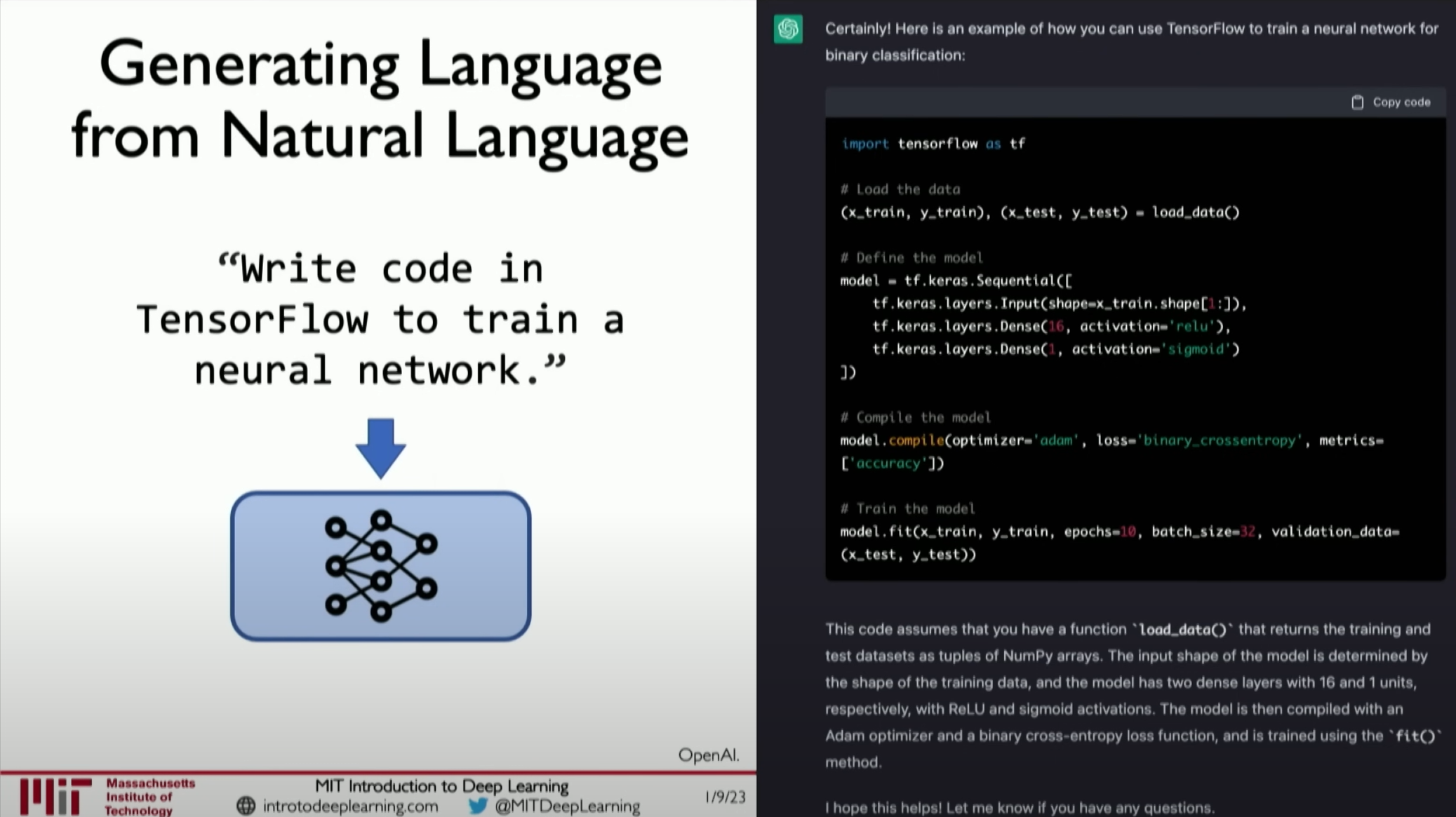
Generating content based on prompts, even generating images that never appear in real datasets, such as a photo of an astronaut riding a horse in space

Generating images or videos based on prompts
Retrieving existing information based on prompts and responding
Building software that generates software
The position of Deep Learning in AI
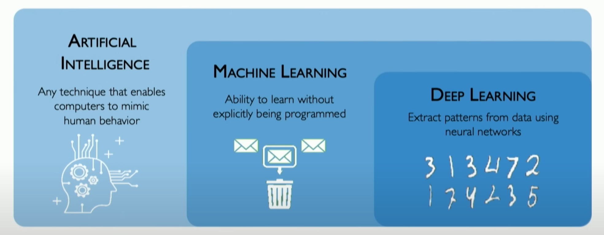
Deep Learning is a subset of Machine Learning that focuses specifically on neural networks and how we can build neural networks that can extract features from data.
Why deep learning?
The evolution from traditional machine learning to deep learning
Traditional machine learning algorithms typically define a set of features in the data, often manually designed based on domain knowledge. Deep learning allows machines to automatically extract and discover core patterns in data, surpassing the limitations of human-defined features. This enables deep learning algorithms to learn higher-level features directly from the data, such as detecting objects like faces by recognizing edges, corners, and curves in images.
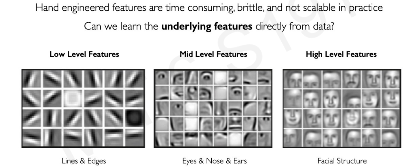
The process of deep learning models detecting objects like faces by recognizing edges, corners, and curves in images involves the following main steps:
Input Image Processing: First, the image is fed as input data to the neural network. These images may undergo preprocessing, such as scaling, cropping, or normalization, to facilitate network processing.Extracting Low-Level Features: The initial layers of the network (usually convolutional layers) start processing the image, detecting basic visual features such as edges and lines. These layers identify low-level features in the image, such as horizontal or vertical edges, by applying different filters (or convolution kernels).Combining Mid-Level Features: As the information passes through the network layers, subsequent layers combine these basic features into more complex shapes and patterns. For example, combining lines and curves to form angles and other geometric shapes.High-Level Feature Recognition: Deeper layers of the network recognize higher-level features such as eyes, nose, and ears. These features are identified based on edges and shapes recognized by previous layers.Face Detection: In the final stage of the network, all detected features are integrated to recognize the entire face. This often involves complex pattern recognition, where the neural network “understands” what combinations of features are most likely to represent a face based on learned features from previous layers.Output and Optimization: Finally, the network outputs its judgment on whether a face is present in the image. During training, this output is compared with actual labels (i.e., whether a face is really present in the image), and network parameters are adjusted based on the difference to improve its future face recognition accuracy.
The entire process is a hierarchical learning process where the neural network builds from low-level to high-level features layer by layer to achieve complex tasks. This capability makes deep learning powerful in image recognition and other fields.
Why Now?
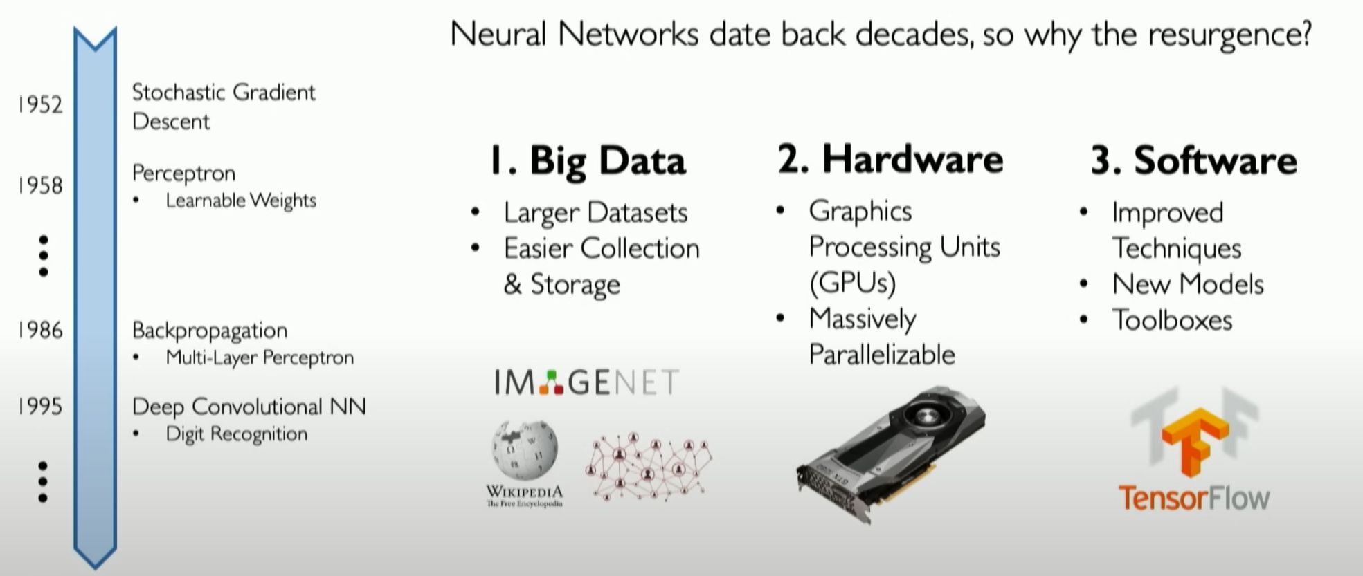
Significant progress in deep learning has been made in the past decade, thanks to several key factors:
The Prevalence of Big Data: We are in the era of big data, providing unprecedented amounts of data for deep learning models, which is crucial for their performance.Large-Scale Parallelization and Computational Power: Deep learning algorithms are highly parallelizable, benefiting from significant advances in hardware that make training large-scale algorithms and techniques feasible, which was previously impractical.Open-Source Tools and Software Platforms: The emergence of open-source tools and software platforms like TensorFlow has made training and coding neural networks easier and more accessible than ever before. This has facilitated wider application and development in the field of deep learning.
The perceptron
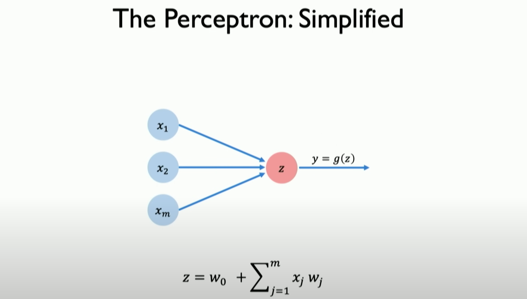
First, we need to know that in a neural network, a single neuron is called a perceptron. I’ll use a diagram to illustrate it simply: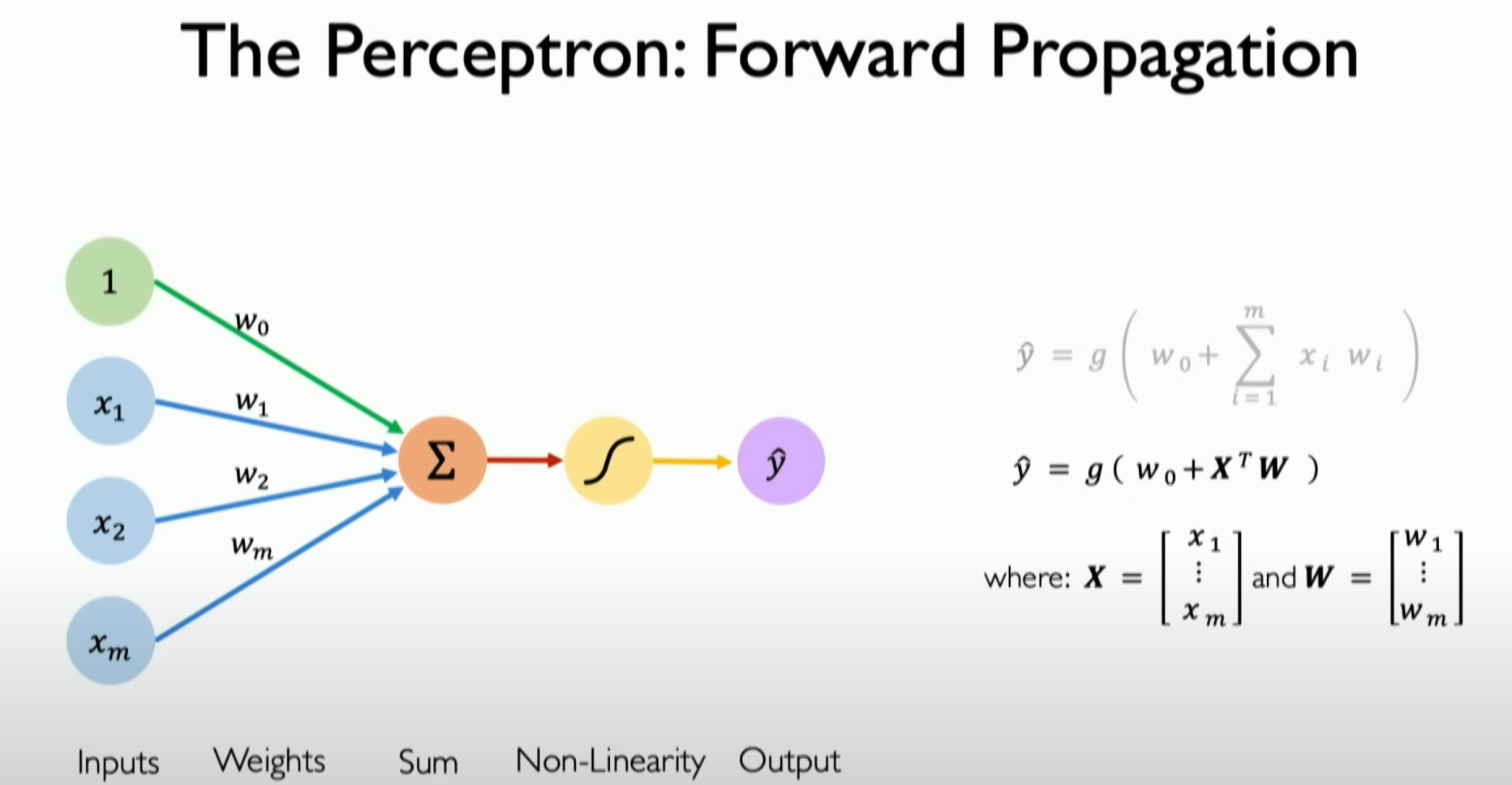
Details of the Perceptron section are as follows:
Perceptron Definition: The perceptron is a basic unit in a neural network, equivalent to a single neuron. It is a fundamental and simple concept in deep learning, primarily used to understand how neural networks work and propagate information.Information Propagation: The core of the perceptron’s work is the forward propagation of information. This process involves three steps: dot product, bias, and non-linearity.Dot Product and Weighted Inputs: To obtain the output of the perceptron, the input is first multiplied by its respective weights. For example, if the perceptron has three inputs X1, X2, and X3, they are multiplied by their respective weights W1, W2, and X3. These product results are accumulated to form a single value.Bias Term: After calculating all the products of inputs and weights, a bias term (usually represented as w0) is added. The bias term is a scalar weight that can be viewed as the weight corresponding to an input always equal to 1. This step is crucial in the perceptron’s operation but is sometimes ignored or simplified.Non-Linear Activation Function: Finally, the sum of the dot product and bias term is processed through a non-linear activation function, resulting in the final output of the perceptron, usually represented as Y. The role of the non-linear activation function is to introduce non-linearity, allowing the network to learn and model complex data patterns and relationships.
The perceptron is one of the most basic building blocks in a neural network. Its working principle involves weighted summation of inputs, bias addition, and non-linear activation. These steps collectively define the forward propagation of information in a neural network.
Why use non-linearity?
I think there’s a lot to talk about regarding non-linear activation functions: Non-linear activation functions play a crucial role in neural networks. Their primary purpose is to add non-linear characteristics to the network, enabling it to learn and model complex data patterns and relationships. Here’s a further explanation of non-linear activation functions:
Why non-linearity?:
Neural networks aim to model complex, non-linear real-world data patterns. Without non-linear activation functions, regardless of how many layers the network has, it can only perform linear transformations, limiting its ability to express and learn complex patterns.
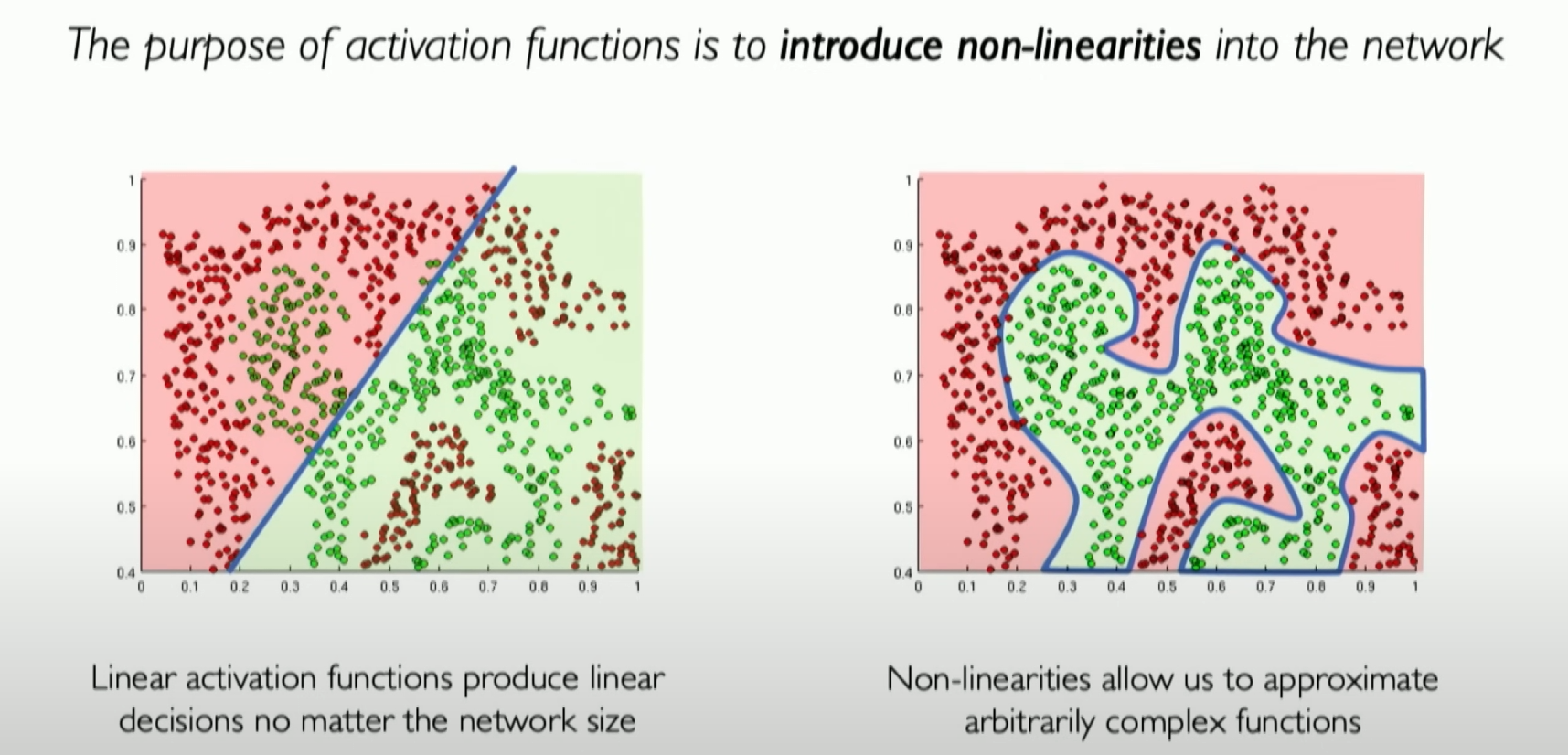
As shown above, we cannot achieve the red-green separation with just a linear boundary, but with non-linear conditions, it can be easily handled.
Non-linear activation functions allow neural networks to establish more complex decision boundaries, enabling them to handle more complex tasks such as image and speech recognition.
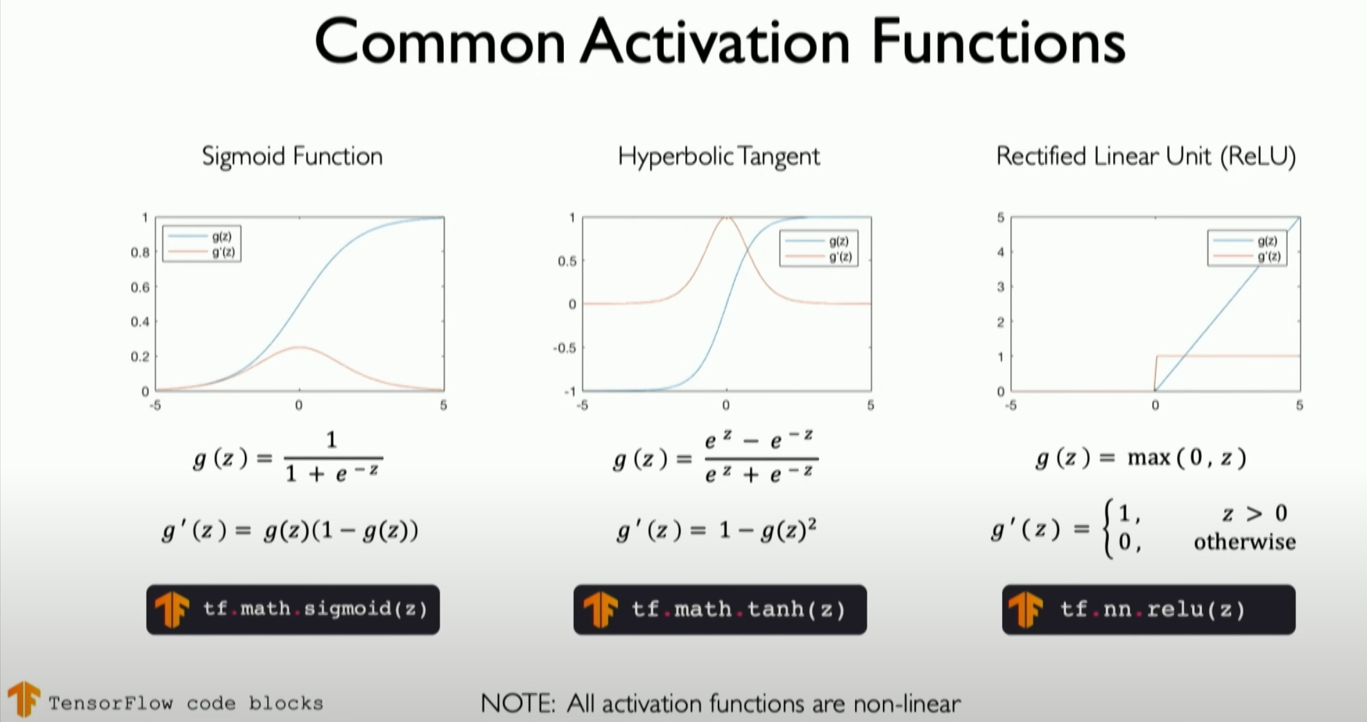
Common Non-linear Activation Functions:
Sigmoid or Logistic Function: This maps any value to the (0,1) range, with the form
. It is often used in the output layer for binary classification. 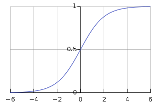
Tanh (Hyperbolic Tangent) Function: Maps input values to the (-1,1) range, with the form
. It has a broader output range than the sigmoid function, usually offering better training performance. ReLU (Rectified Linear Unit) Function: With the form
, it remains linear in the positive range and outputs zero in the negative range. ReLU is widely used due to its simplicity and effective training performance. We will detail it in later chapters.
The Role of Activation Functions:
- Activation functions determine whether a neuron should be activated, helping neurons decide what information is important and should be further transmitted.
- They introduce non-linearity, enabling the network to handle more complex and abstract problems.
Choosing Activation Functions:
- The choice of a specific activation function depends on the application and network architecture. For example, the sigmoid function is
commonly used in the output layer for binary classification problems.
- ReLU and its variants (e.g., Leaky ReLU, Parametric ReLU) have become popular due to their effectiveness in training deep networks.
Challenges with Activation Functions:
- Some activation functions (e.g., sigmoid and tanh) may lead to the “vanishing gradient” problem, slowing down learning in deep networks.
- Although ReLU is effective, it has the “dying ReLU” problem, where some neurons might never activate, causing information loss.
In summary, non-linear activation functions are a key part of neural network design, allowing the network to learn various data patterns from simple to complex. Properly selecting and using activation functions is crucial for building effective neural network models.
From perceptrons to neural networks
Now, let’s review the previous content and re-establish the concept of Perceptron.
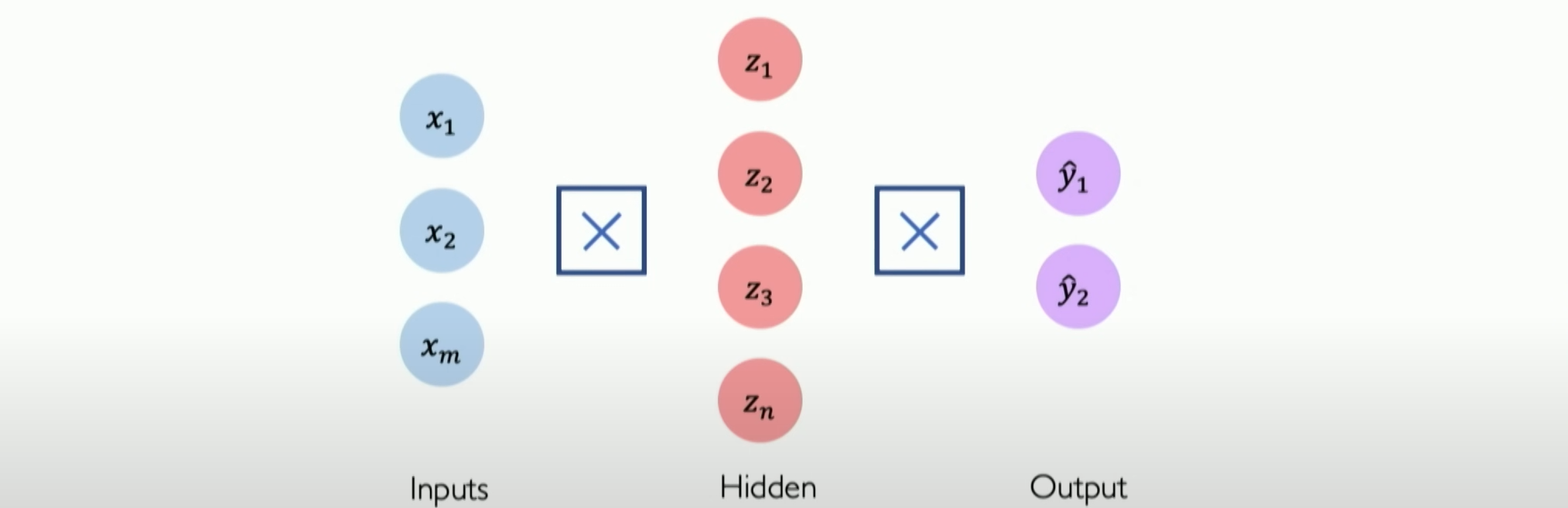
For simplicity, we don’t draw the weight and bias, but they still exist. Now, the result is Z, which we call the result of the dot product plus bias. This is what we pass to the non-linear function g, the activation function g about z.
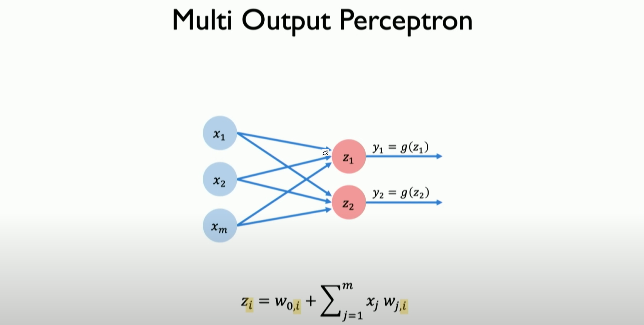
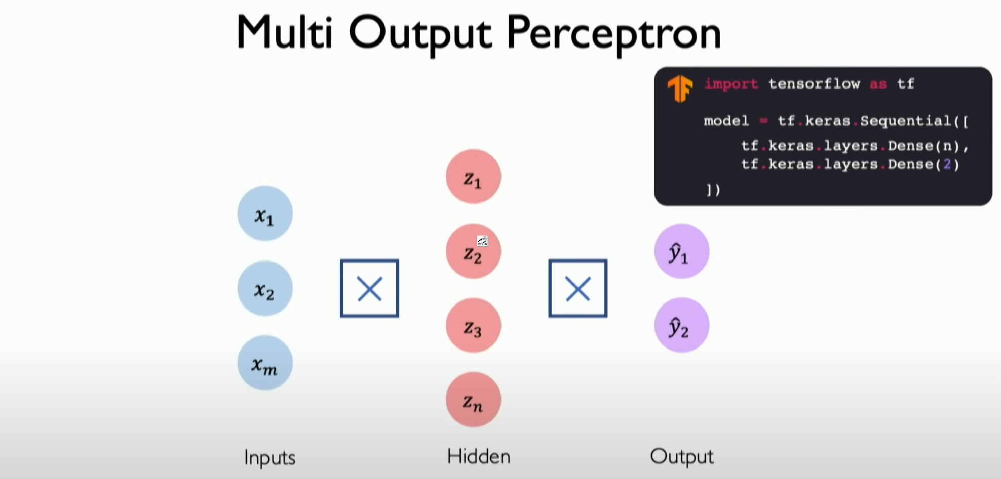
If we want to define and build a multi-layer output neural network, as shown in the above figure, with two outputs, it is still the result of the dot product plus bias. The two perceptrons corresponding to the two neurons will control the output of their associated parts.
With the above mathematical understanding, we can convert it into code. Here, we use TensorFlow and Keras to build our dense layer (Dense Layer) for implementing custom forward propagation, which is our perceptron:
1 | import tensorflow as tf |
First, the first part initializes our weight vector. The second part is our bias vector. Next, we dot product all our inputs with our weights and add bias, then pass it through a non-linear function (activation function) to return the result. This is what the call function does. This code will run and define a complete neural network layer, then you can use it like this:
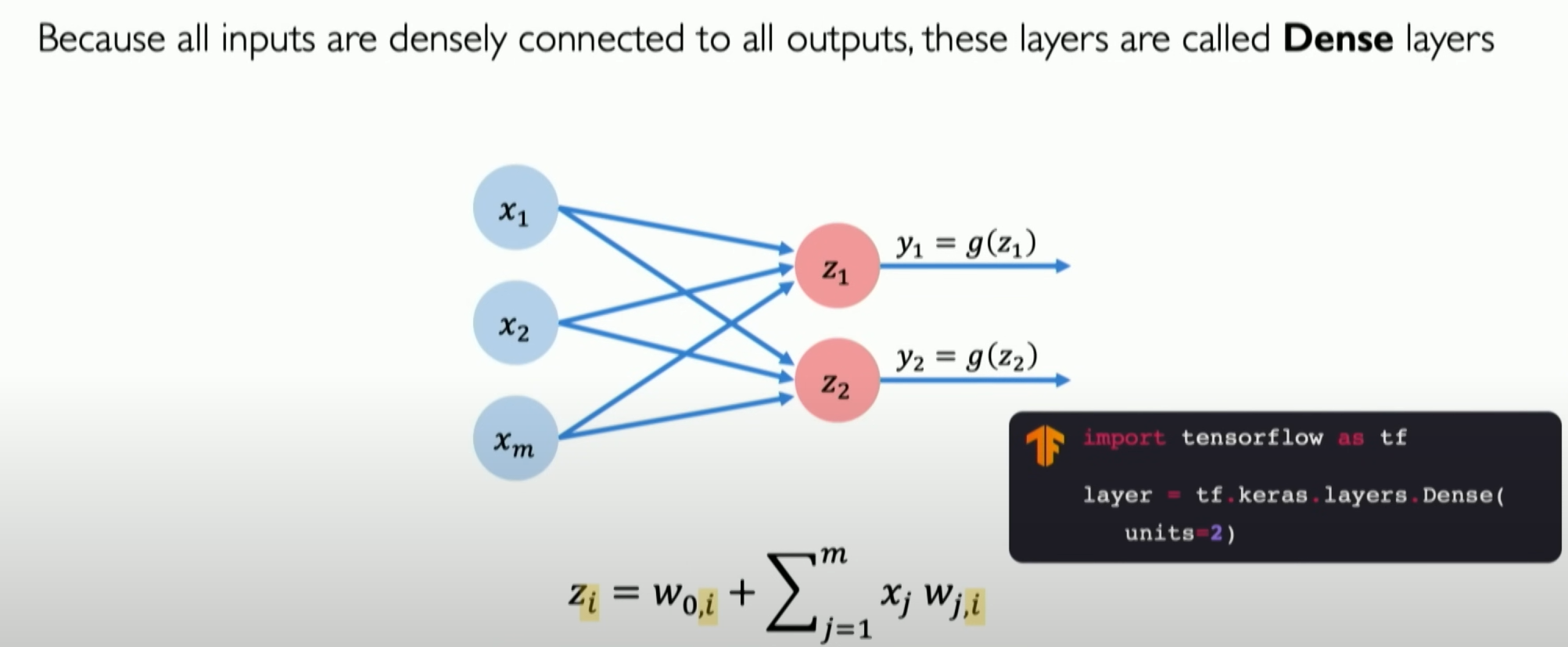
In practical TensorFlow usage, we only need to call it directly as shown above.
Stacking Layers
Now, we can officially consider how to stack these layers to form a neural network.
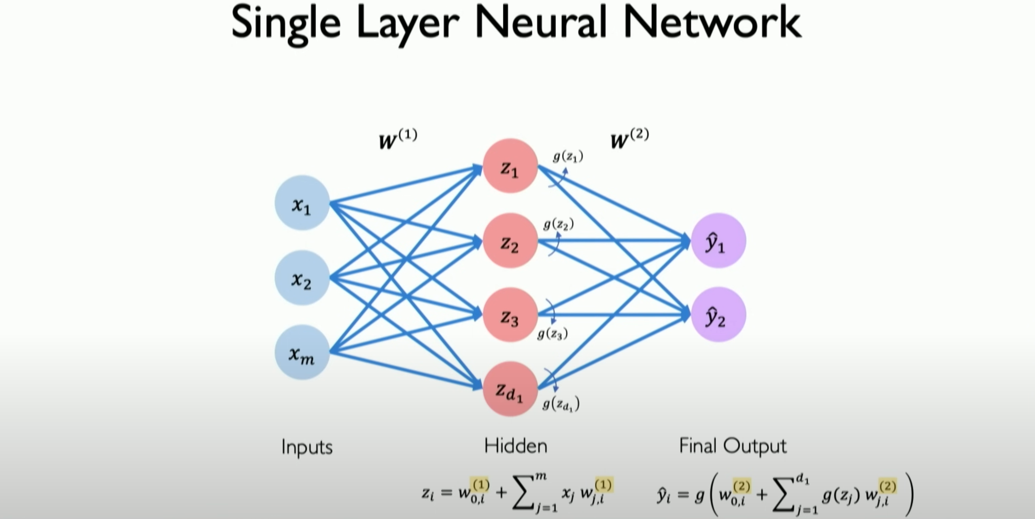
Now, let’s only look at a single-layer neural network.
Let’s simplify all the lines to show only the icons in the middle, proving that everything is fully connected. This covers all the previously mentioned mathematical equations without adding any complexity. Well, with this type of solution, we can consider how to stack layers on top of each other to create so-called sequential models.
Sequential models basically define the forward propagation of information, not only at the neuron level but now extending to the layer level. Each layer will be fully defined and connected to the next layer. The input of the next layer will be the output of all previous layers, introducing deep neural networks on this basis.
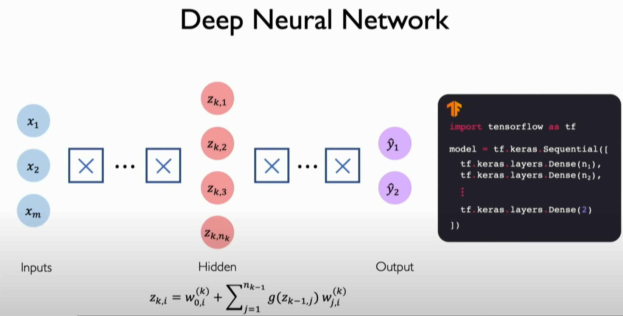
This is no different from before, except that these layers are stacked continuously, correctly calculating the final output through more in-depth understanding of different layers, eventually reaching the last layer, i.e., the output layer, which is the final result we want to output.
Loss functions
First, we need to introduce the concept of the loss function with the help of an example.
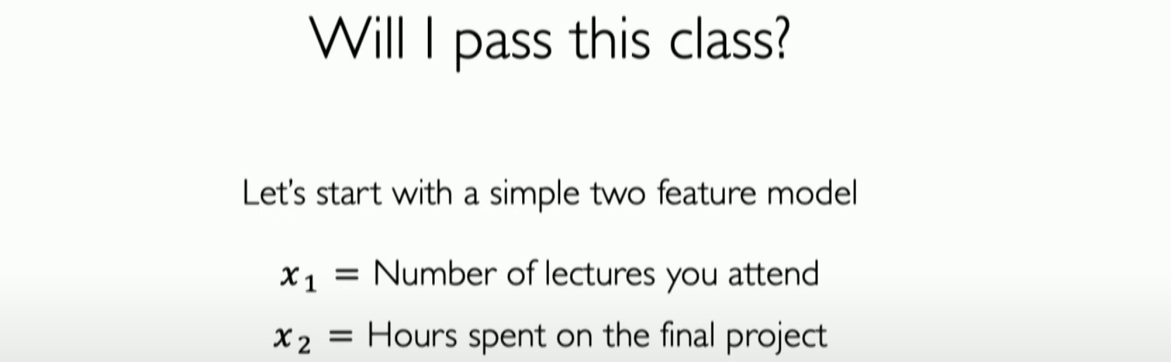
Let’s try to establish a neural network to judge whether you can pass a course. It has only two inputs: x1 is the number of lectures attended, and x2 is the time spent on projects.
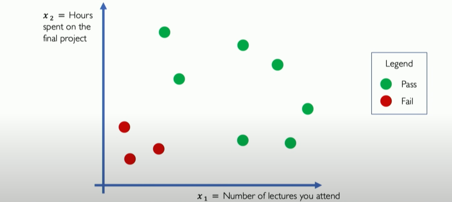
We can see from the above figure that over the past few years, students’ data have been plotted on this two-dimensional feature map of the input space, showing the relationship between the two and the final pass or not.
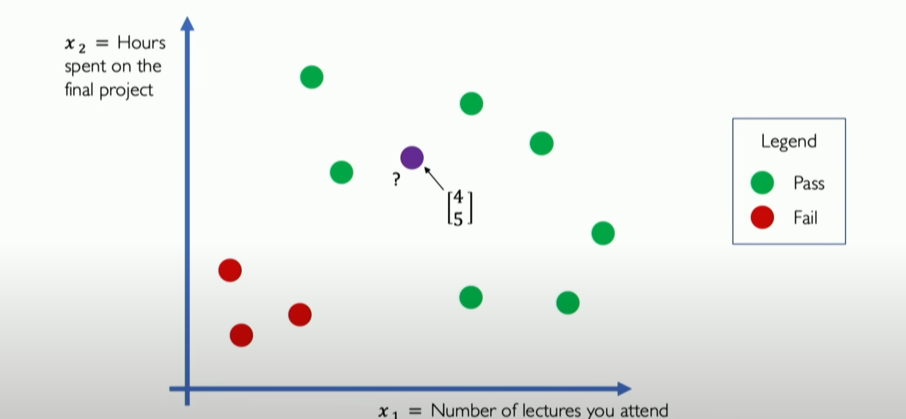
Assume [4,5] is your coordinate, and you want to predict whether you will pass the class through the neural network. Now we abstract out the neural network diagram:
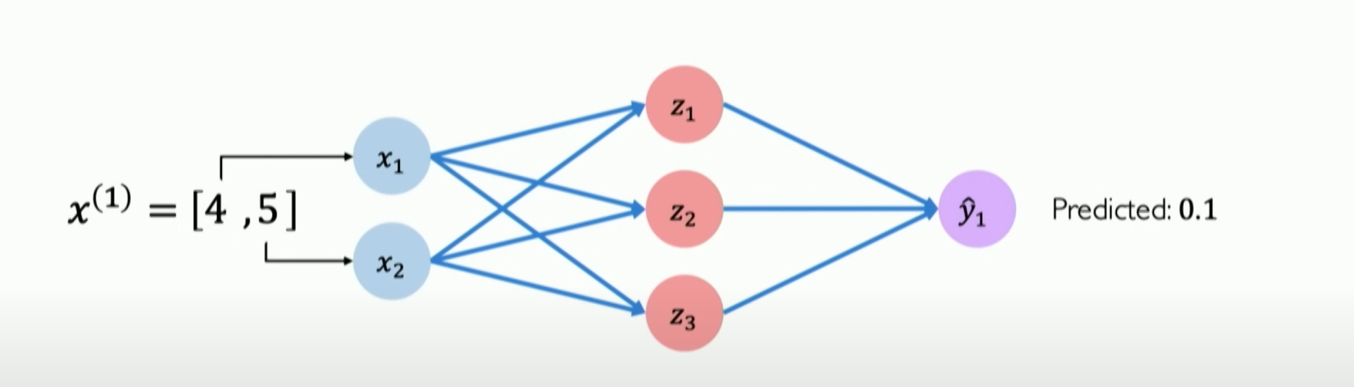
But we find that our pass rate is only 0.1 after the neural network prediction. Why? Obviously, we can see that our position is in the high probability pass range in the two-dimensional feature map of the data.
The reason is simple: this neural network has not been trained with any datasets. It is like a blank sheet of paper; it does not know what passing or failing means.
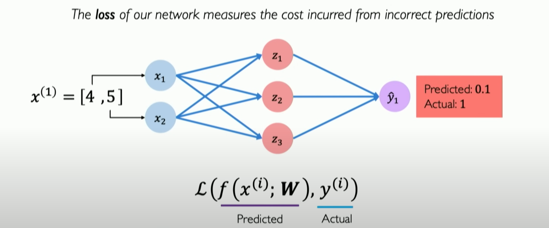
So, we need to start training it, and part of this understanding is that we first need to tell the neural network when it makes a mistake. Mathematically, we need to tell it how big its mistake is when it makes a mistake, so it can better minimize the mistake the next time it sees this data point. In neural networks, these mistakes are called losses.
Specifically, we need to define a loss function that takes your prediction and the actual prediction as input and tells you how far apart they are, i.e., how big of a loss there is.
Our ultimate goal is to minimize the average mistake our neural network makes on all mistakes.
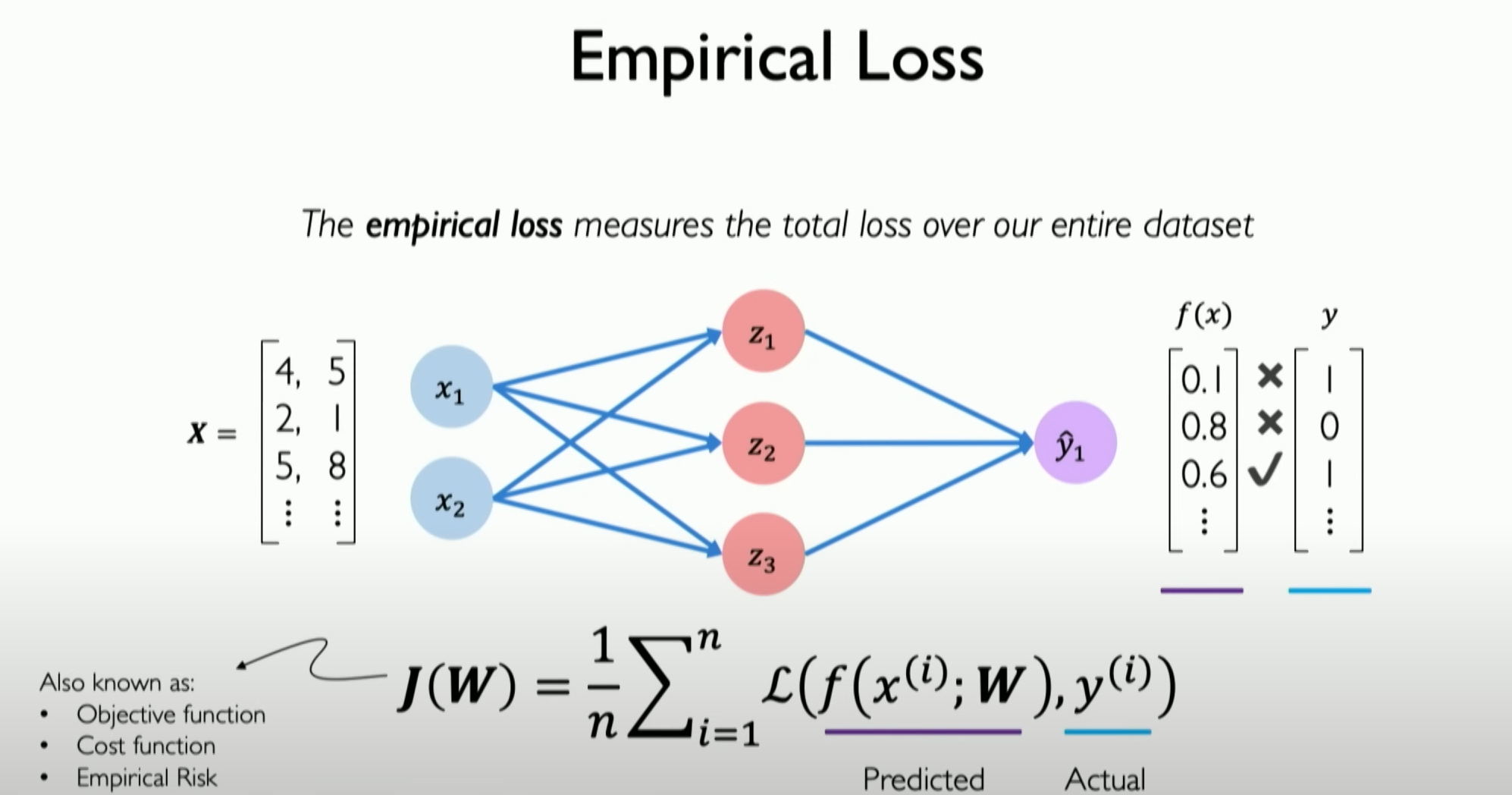
Definition of Loss Function:
- In neural networks, the loss function (also known as the objective function, empirical risk, or cost function) measures the difference between the model’s predicted values and the actual values. It is an important tool for evaluating model performance and guiding the network training process.
Types of Loss Functions:
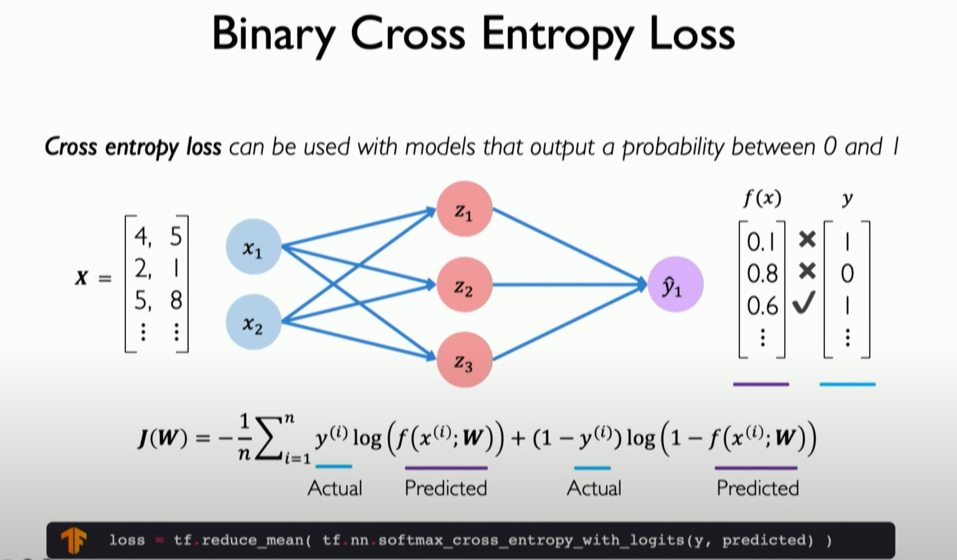
Binary Classification Problems: For binary classification problems, the commonly used loss function is softmax cross-entropy loss.
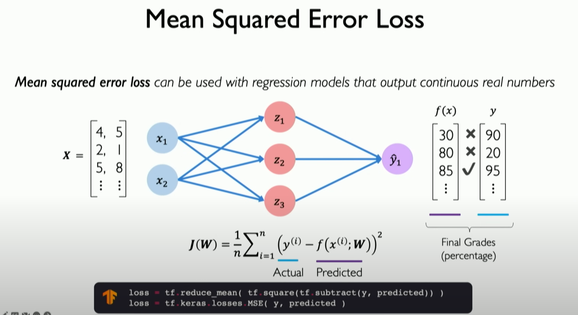
Other Problems: For other types of problems, different loss functions may be used, such as mean squared error for regression problems.
Goal:
The goal of training a neural network is to find a set of weights (W) that minimize the average value of the loss function across the entire dataset.
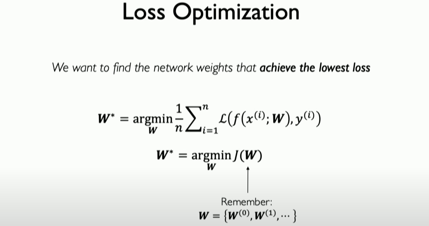
Here, W is just a list, representing a set of all weights in our neural network.
Loss functions play a crucial role in neural network training. They provide a way to measure model performance and guide the model to improve through gradient descent or other optimization algorithms. Different types of problems may require different loss functions, and choosing the right loss function is essential for training effective neural network models.
Training and gradient descent
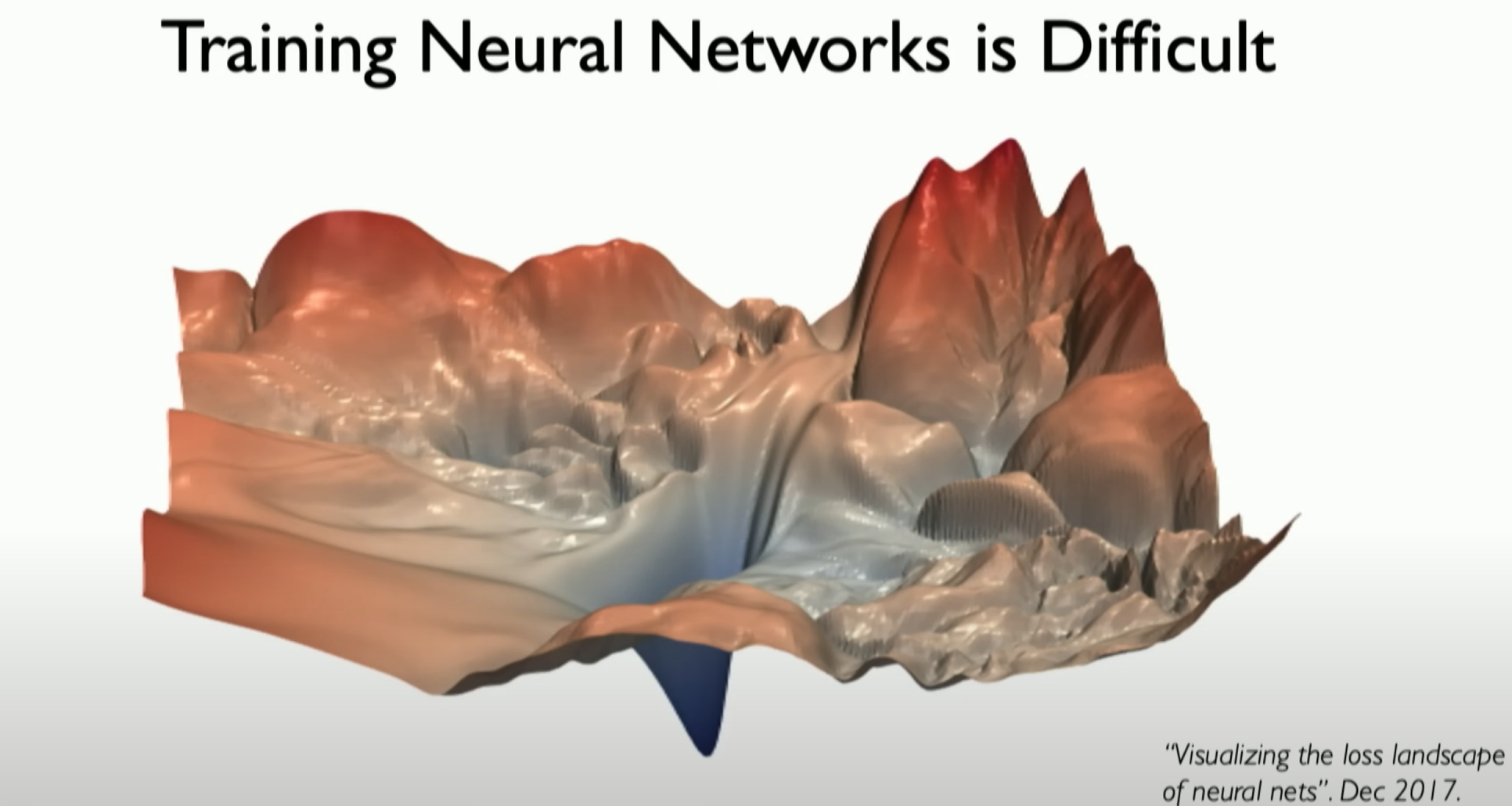
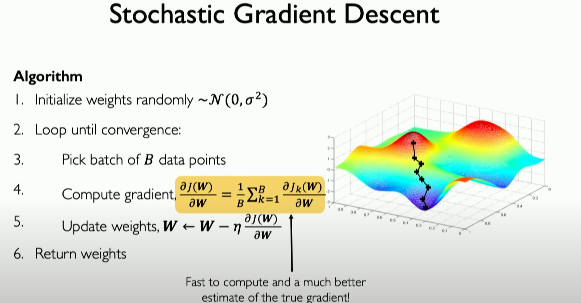
Before introducing the gradient descent algorithm, we need to visualize a simple three-dimensional distribution of loss to understand that calculating the gradient on the entire dataset is
not feasible when the dataset is large. So, we must find an alternative method, which introduces the concept of batched gradient descent.
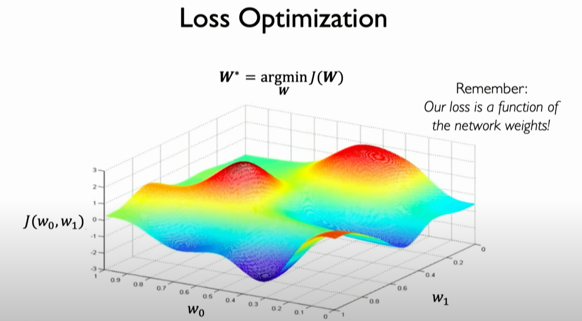
Initially, we start from a random place in space. We can calculate the loss at this specific position, and more importantly, we can calculate how the loss changes from this point. We can calculate the gradient of the loss, and because our loss function is continuous, we can actually calculate the derivative of the loss function in the weight space. The gradient tells us the direction of the highest point.
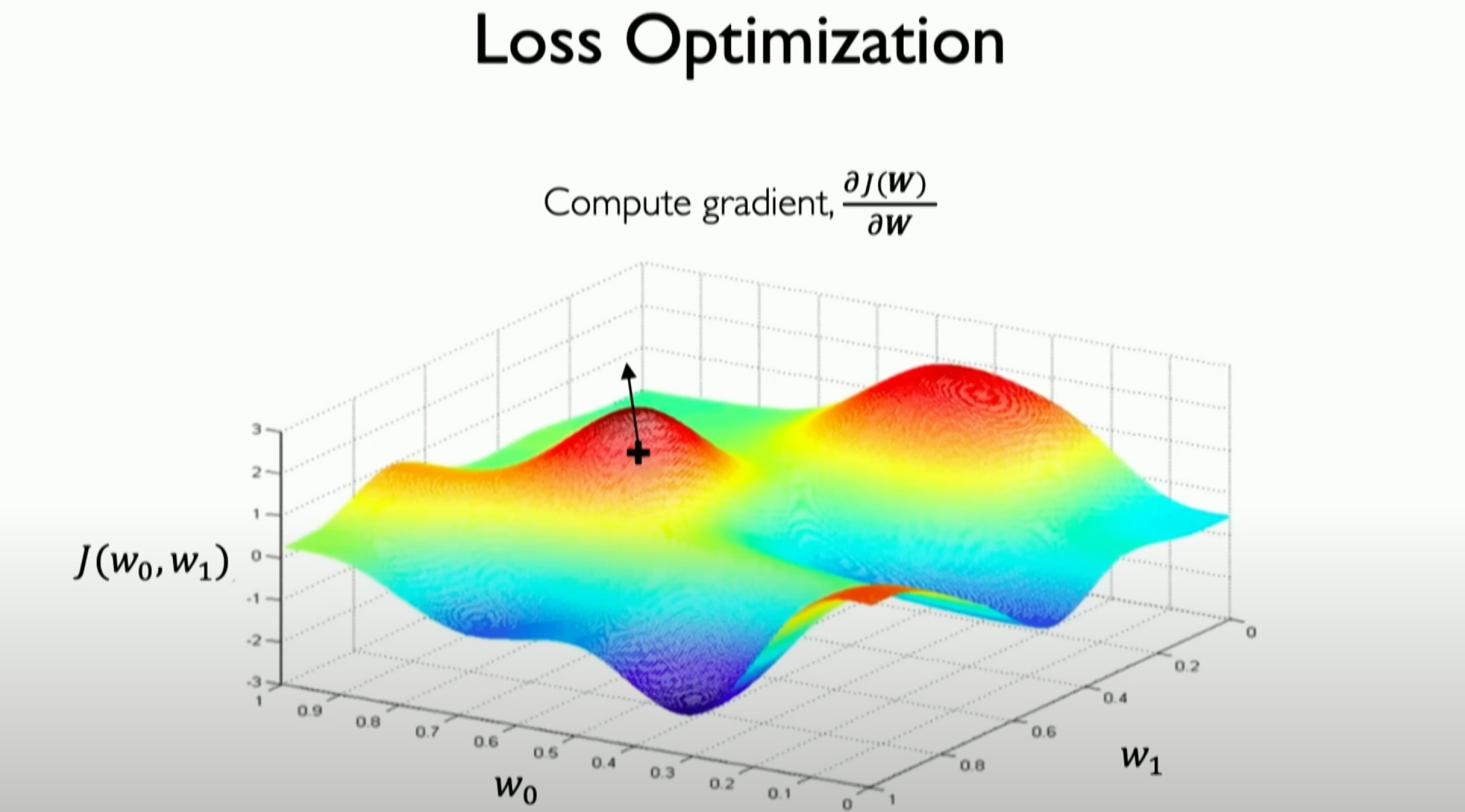
From our current position, the gradient tells us which way will increase our loss, so we actually take a step in the opposite direction of the gradient.
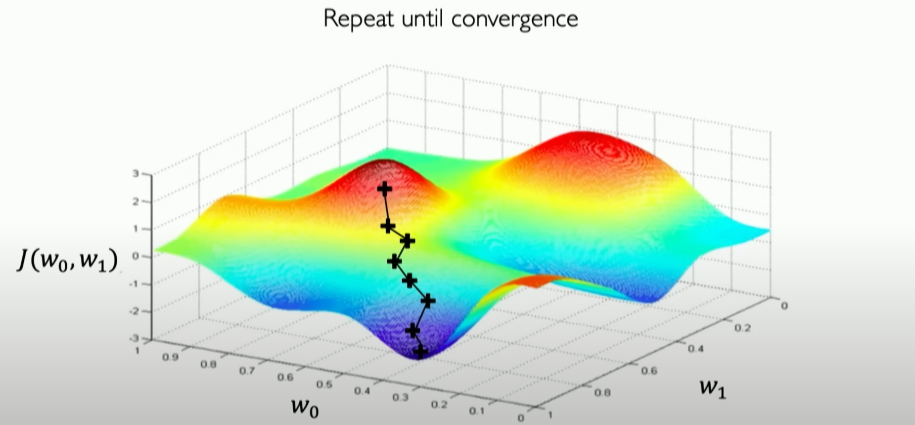
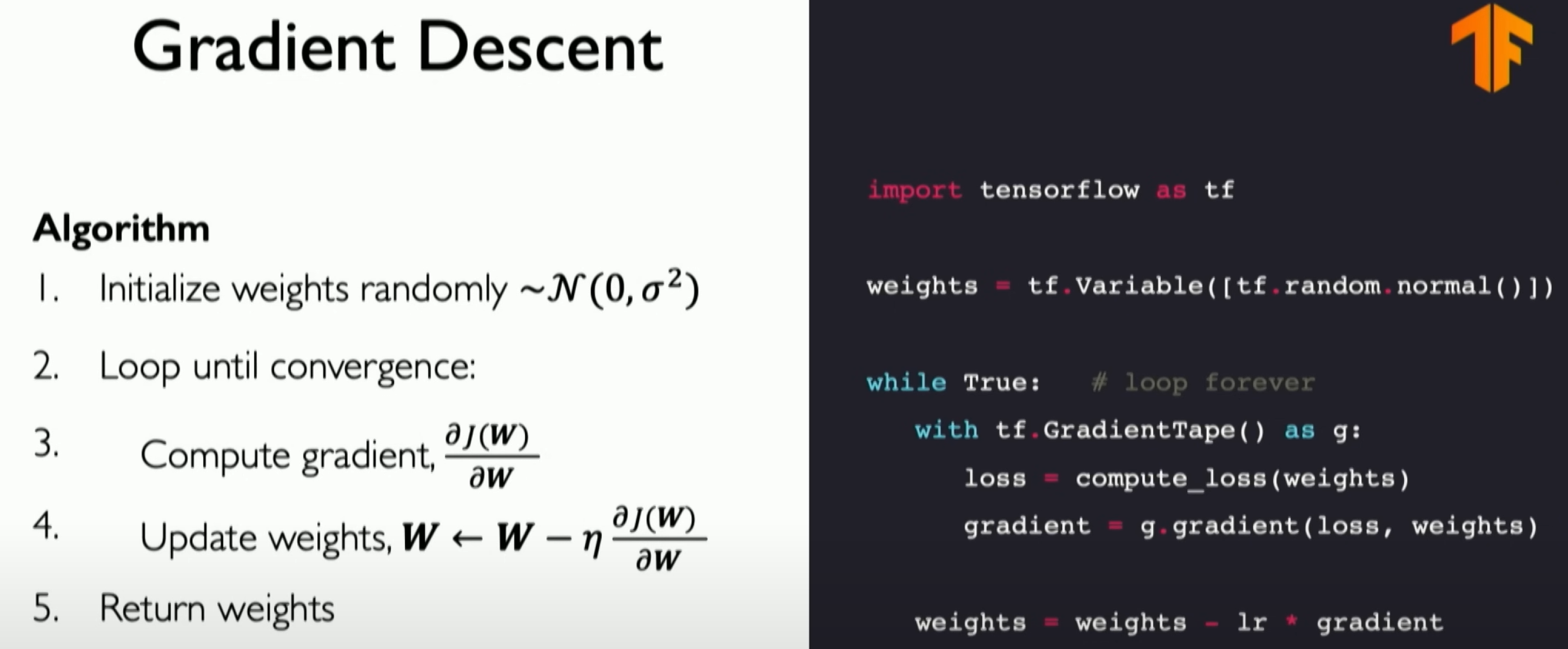
Then we repeat this process until our loss converges to a minimum value. Now we can summarize the entire gradient descent algorithm:
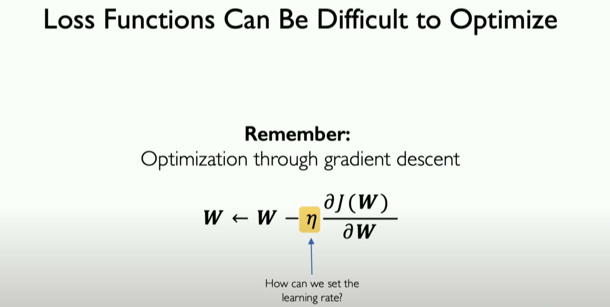
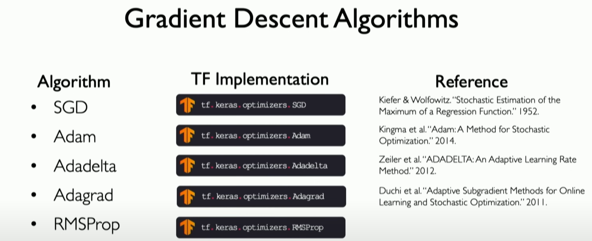
Gradient Descent:
Gradient descent is an optimization algorithm used to minimize the loss function of a neural network.
The process starts with random initialization of weights and then gradually adjusts the weights to reduce the loss.
We calculate the gradient of the loss and update our W (set of weights) in the opposite direction of this gradient. The goal is to find the weight combination that minimizes the loss.
Stochastic Gradient Descent (SGD):
- In practice, stochastic gradient descent (SGD) is used instead of traditional gradient descent. SGD uses only one sample or a small batch of samples from the dataset to calculate the gradient at each iteration, speeding up calculations and reducing memory requirements.
- Although SGD introduces randomness, it can converge faster and help avoid local minima.
Learning Rate:
- The learning rate is an important parameter in gradient descent, determining the step size for weight updates.
- Proper learning rate selection is crucial for fast convergence and avoiding overfitting.
Mini-batch Gradient Descent:
- Mini-batch gradient descent is a compromise between traditional gradient descent and SGD, using a subset of the dataset (e.g., 100 data points) to calculate the gradient at each iteration.
- This method balances computational efficiency and gradient estimation accuracy.
Loss Function Calculation:
- The goal of training a neural network is to minimize the loss function, which measures the difference between the model’s predictions and actual labels.
- Different types of neural networks and tasks may require different loss functions.
Backpropagation
Now we must introduce the concept of Backpropagation because the backpropagation algorithm is a key step in calculating gradients in gradient descent.
Backpropagation:
Backpropagation is a key step in calculating gradients in gradient descent. It is based on the chain rule and involves passing the error from the output layer back to the input layer to update the weights effectively.
Through backpropagation, each weight update is based on its contribution to the final output error.
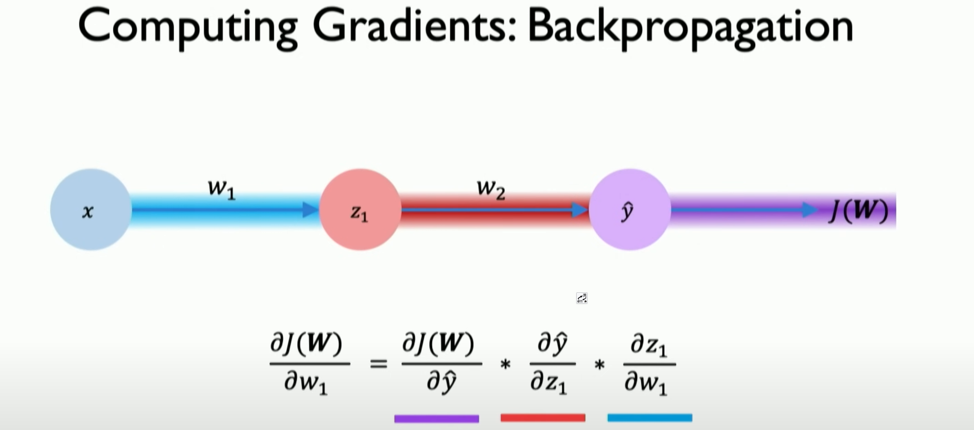
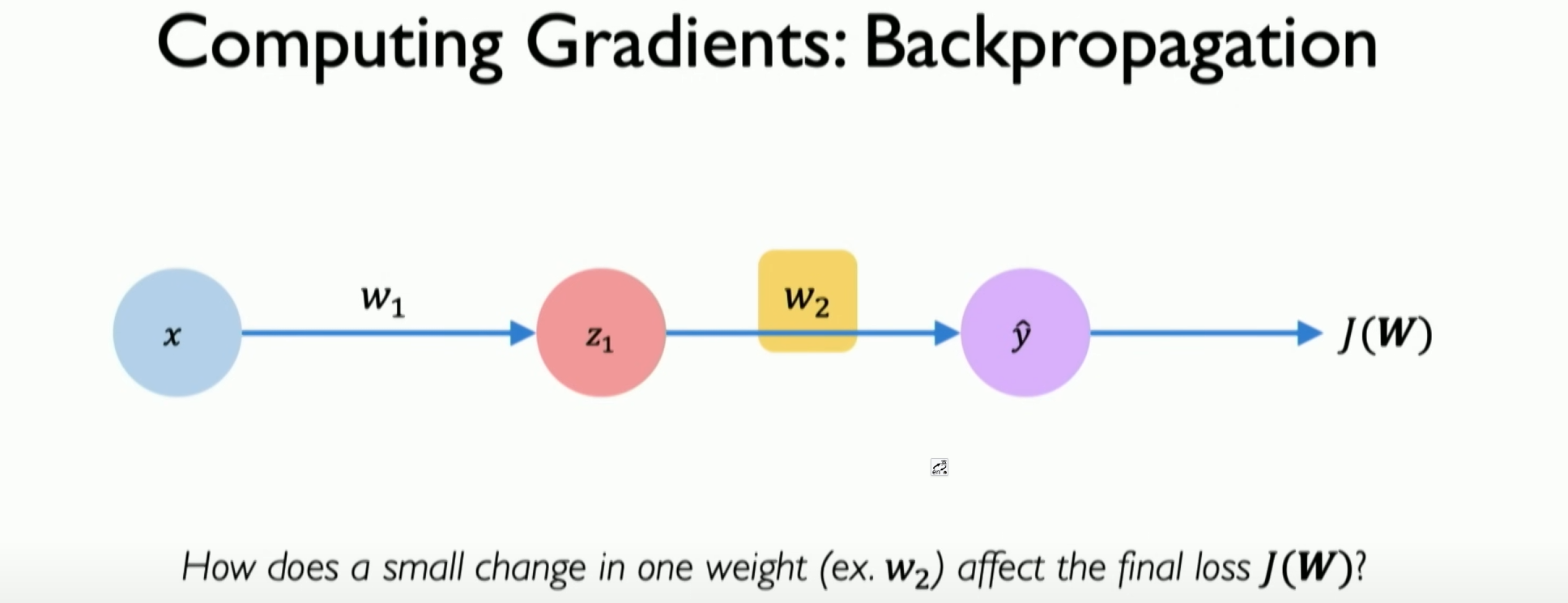
We can illustrate this process through the chain rule. It can determine how each weight and small changes in these weights can increase or decrease the impact on our loss function. This is the backpropagation algorithm, the core of training neural networks.
Gradient Calculation and Propagation:
- At the level of a single neuron or perceptron, the derivative related to the weight (e.g., W2) is first calculated.
- Then, these gradients are backpropagated through the network to the input layer to update the relevant weights.
Role of Learning Rate:
The learning rate is an important parameter that determines the step size for weight updates at each iteration, i.e., the step size in the opposite direction of the gradient.
A too high learning rate may lead to over-adjustment, and too low a learning rate may slow down training.
Relationship Between Forward Propagation and Backpropagation:
- Forward propagation is the process of passing information from the input layer to the output layer.
- Backpropagation is the process of passing the error from the output layer back to the input layer to update the weights.
Sequential Models and Layer Structures:
- Neural networks can be constructed as sequential models, where each layer is fully connected to the next.
- In this structure, the output of each layer becomes the input for the next layer, forming a hierarchical forward propagation path.
Implementation of Backpropagation:
- The backpropagation algorithm can be directly implemented in various deep learning frameworks, such as TensorFlow or PyTorch.
- It typically includes calculating the gradients of the loss function and using these gradients to update the weights in the network.
Complexity of Backpropagation:
- Although theoretically simple, backpropagation can be very complex in practice, especially when dealing with large networks and complex datasets.
Training Neural Networks:
- Backpropagation is part of training neural networks, including applying the model to the dataset, optimizing weights through backpropagation, and learning various tips and techniques to improve training efficiency.
In practical training, optimizing a neural network looks more like this:
Setting the learning rate
Role of Learning Rate:
- The learning rate is an important parameter that determines the step size for weight updates at each iteration, i.e., the step size in the opposite direction of the gradient.
- A too high learning rate may lead to over-adjustment, and too low a learning rate may slow down training.
Finding the minimum loss above is very difficult, and the
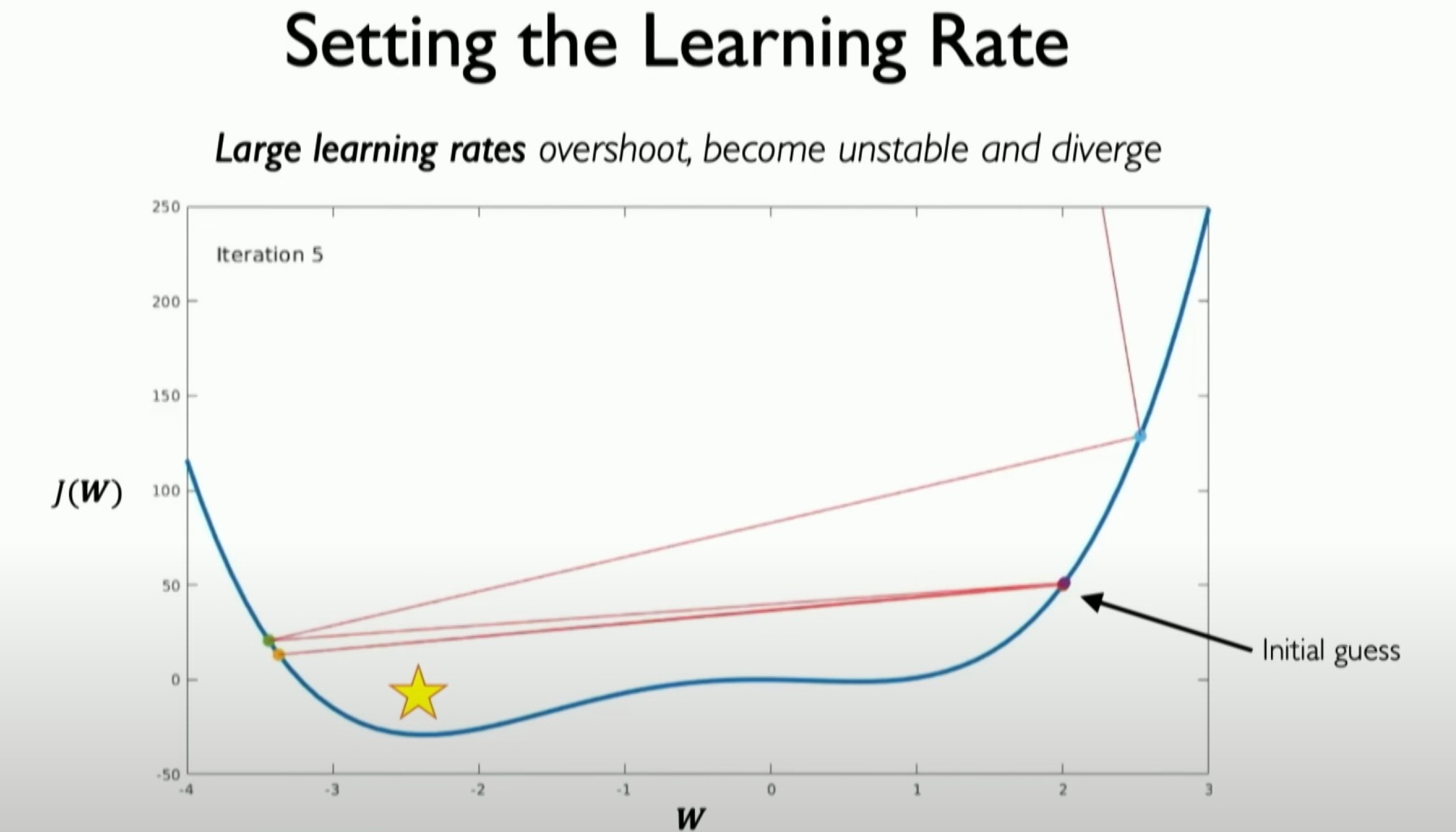
When the learning rate is too high, convergence is difficult, and even deviations in the solution direction may occur.
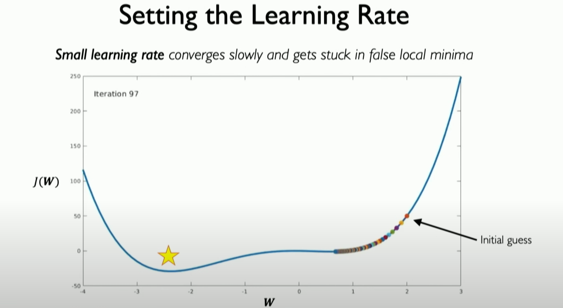
When the learning rate is set too low, it is easy not to converge at the best point.
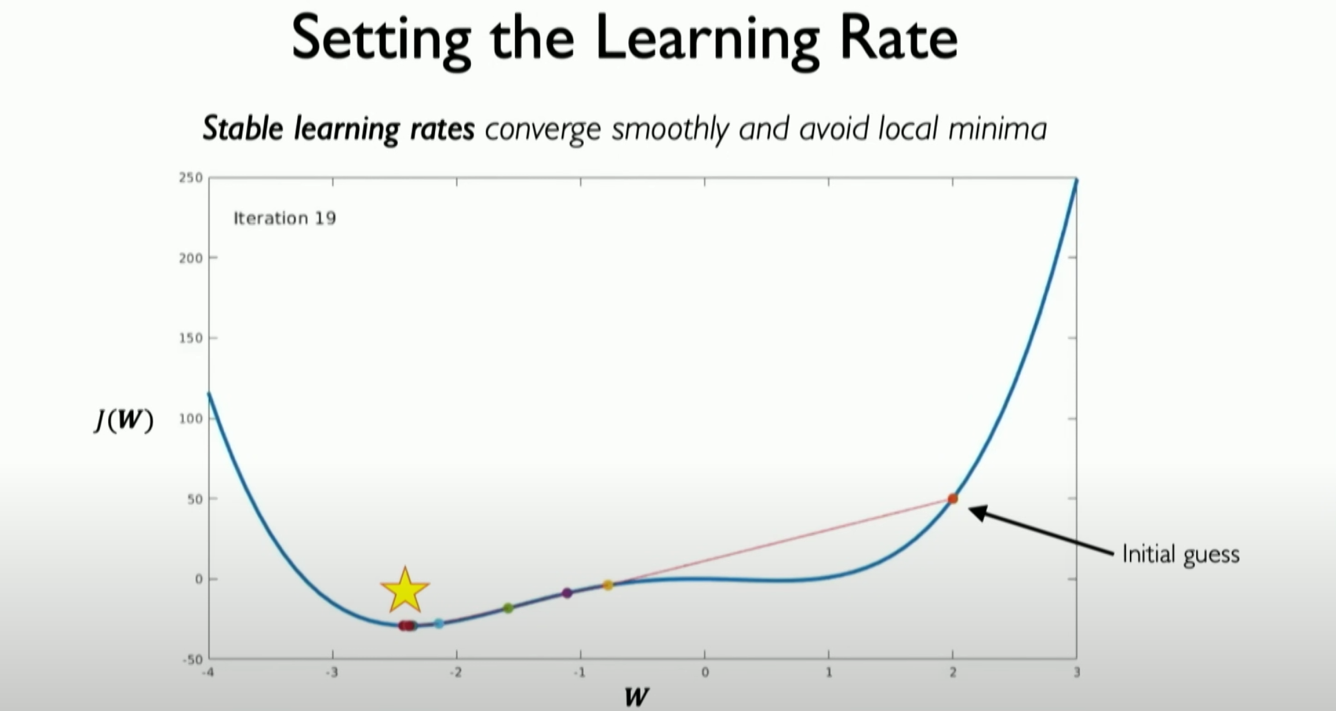
We expect it to go beyond the local minimum value, enter the reasonable part of the search space, and thus converge to the expected position we are most concerned about.
We can think of two ways to solve this problem: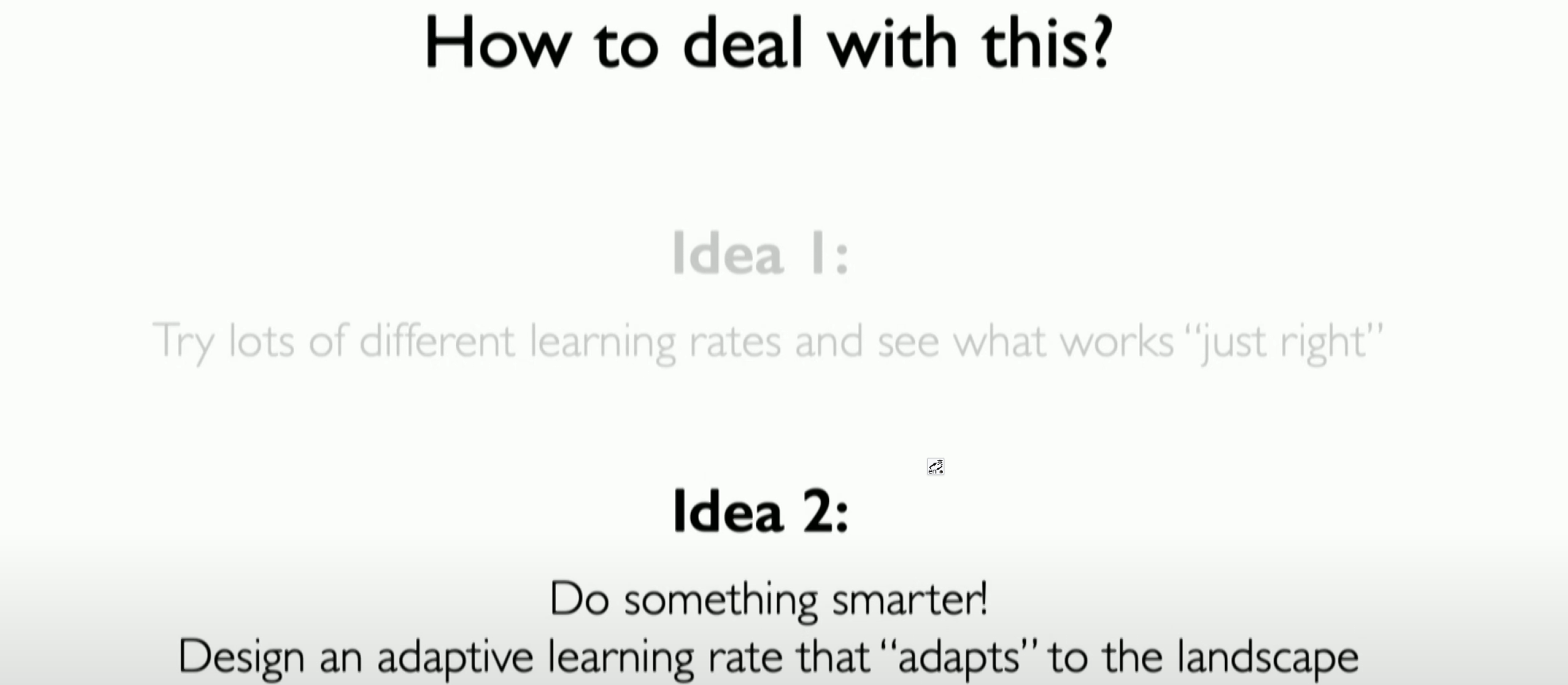
One is to continuously try different learning rates
More specifically, this ultimately means that the learning rate (i.e., the speed at which the algorithm trusts the observed gradient) will depend on several factors:
- Size of the Gradient: The size of the gradient at a specific location affects the learning rate. If the gradient is large, it may indicate that a larger learning step is needed to quickly adjust the weights.
- Speed of Learning: The speed of learning, i.e., the speed of updating network weights, also affects the choice of learning rate. Fast learning may require a higher learning rate to quickly utilize large gradients for adjustment.
- Other Options: There may be various other factors and options affecting the setting of the learning rate, such as the choice of optimization algorithm, the complexity of the network structure, etc.
The details of the learning rate are as follows:
- `Impact of Too
High Learning Rate`:
- If the learning rate is set too high, it may cause overshooting, i.e., the neural network deviates from the solution, and the gradient may explode, leading to performance degradation.
Challenges of Learning Rate:
- In practice, determining the appropriate learning rate is a challenge as it significantly affects the training and performance of the neural network.
Smarter Learning Rate Setting:
- Instead of simply trying different learning rates, a learning rate algorithm that can adapt to the characteristics of the neural network can be designed to more intelligently adapt to the network’s training process.
Impact of Too Low Learning Rate:
- Setting the learning rate too low will slow down the learning speed and may even fail to converge to the global minimum because the network may get stuck in local minima.
Adaptive Learning Rate Algorithms:
Various adaptive learning rate algorithms exist that have been widely researched and applied in practice. Additional details: Optimizing Gradient Descent
Learning Rate and Gradient Descent Update Equation:
- The learning rate determines the step size of the gradient descent iteration in backpropagation.
Possibility of Increasing Learning Rate:
- Averaging gradients over batches can improve gradient accuracy, allowing for an increased learning rate and faster learning speed.
Relationship Between Learning Rate and Gradient Accuracy:
- Improved gradient accuracy allows faster convergence to the solution and may enhance the efficiency of the learning rate.
Practical Application of Learning Rate:
- In practical applications, the learning rate is usually defined with the optimizer to control the speed and direction of weight updates.
At this point, we can take a break and integrate all the previously mentioned information into our code implementation.
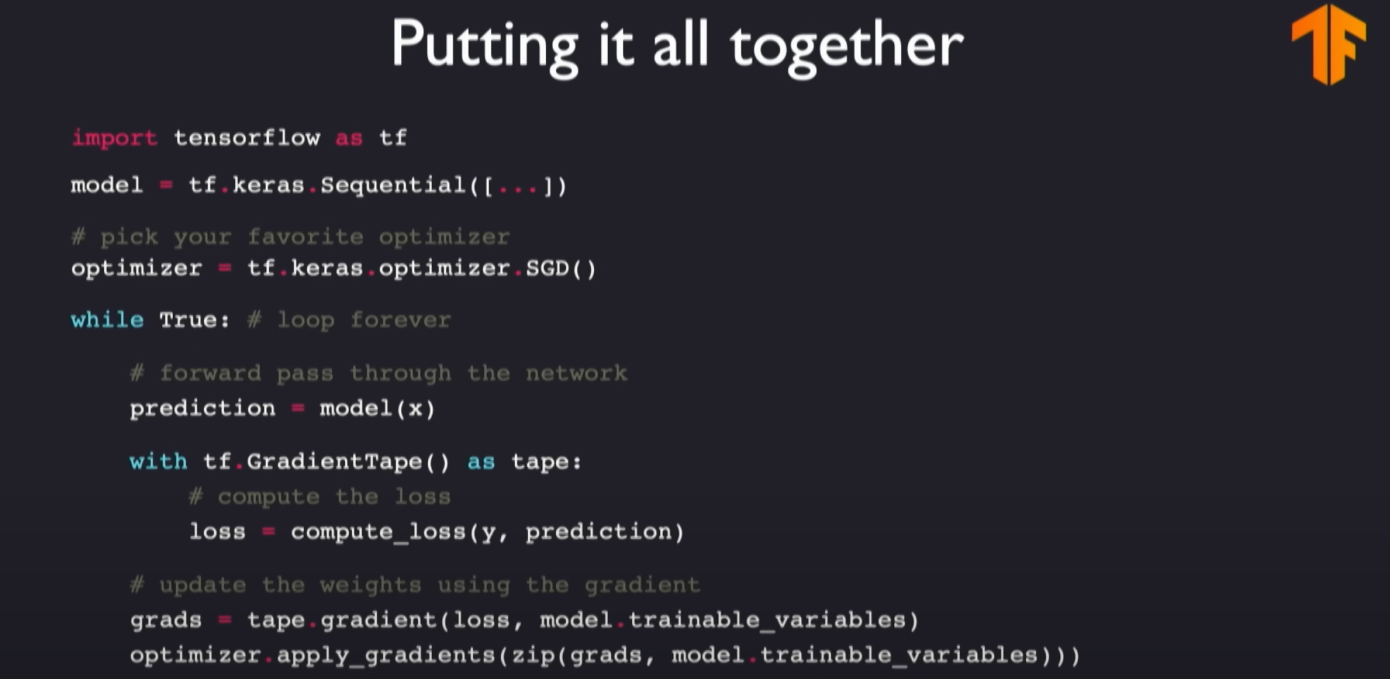
The steps in the above diagram include:
Model Definition: First, define the model at the top level of the neural network. This involves constructing and setting up the structure of the neural network, as discussed earlier in the lecture.Optimizer and Learning Rate: Next, define the optimizer for each part of the model. The optimizer is set together with the learning rate, which determines the speed of optimizing the loss function.Iterative Training Process: In multiple training loops, the model iterates over all samples in the dataset. This process involves observing and understanding how to improve the neural network.Gradients and Network Improvement: Next, improve the network based on gradients. Gradients indicate the direction in which network weights need to be adjusted.Continuous Optimization: This process continues until the neural network gradually converges to a solution.
Batched gradient descent
When reviewing the implementation process of the gradient descent algorithm, we can see that calculating the gradient on the entire dataset is not feasible when the dataset is large. Therefore, we must find an alternative method, introducing the concept of batched gradient descent, which involves calculating the gradient using only a part of the sample data. Although this will have a lot of noise, the calculation speed will be much faster.
This formula is used to calculate the average gradient of weights (W) in mini-batch gradient descent. Let’s analyze this formula step by step:
- Definition of Gradient:
represents the gradient of the loss function with respect to the weights . This gradient indicates the rate at which the loss function changes with the weights, guiding weight updates.
- Average Gradient of Mini-Batch:
is the average value of all sample gradients in a mini-batch, where is the batch size, representing the number of samples in the mini-batch. represents the gradient of the loss function with respect to the weights for the -th sample.
- Calculation Process:
- First, for each sample (
from 1 to ), calculate the gradient of the loss function with respect to the weights. - Then, sum these gradients and divide by the batch size
to obtain the average gradient of the entire batch.
- Optimization and Updates:
- This average gradient is used to update the weights in the optimization process. By applying this average gradient, weights can be adjusted more smoothly, reducing the randomness and noise that individual sample gradients might bring.
- Efficiency and Accuracy:
- By calculating the average gradient over mini-batches, this method combines the computational efficiency of stochastic gradient descent with the accuracy of full-batch gradient descent.
Overall, this formula is the core of the mini-batch gradient descent method. It updates the weights in the neural network by calculating the average gradient of all samples in the mini-batch. This method reduces computational burden while improving the accuracy of gradient estimation.
The details of batched gradient descent are as follows:
Concept of Batch Data:
- Batched gradient descent involves dividing the data into mini-batches, each containing a small portion of the dataset.
- This method is an improvement on the gradient descent algorithm, aiming to reduce computational costs and improve efficiency.
Computational Efficiency and Gradient Accuracy:
- Calculating the gradient over the entire dataset is very computationally intensive. Batched gradient descent reduces this computational burden by using only a mini-batch of the dataset to calculate the gradient.
- Using mini-batches significantly reduces randomness compared to single samples (stochastic gradient descent) and improves gradient accuracy.
- Batch sizes typically considered are between tens to hundreds of data points. Such sizes are much faster to compute than the gradient of the entire dataset while being more accurate than gradient calculations based on single samples.
Performance and Convergence:
- Batched gradient descent balances computational efficiency and gradient estimation accuracy, providing more stable performance and convergence behavior during training.
- This method allows for faster iterations and avoids extreme changes in gradient descent algorithms during training.
Practical Applications:
- In practical applications, batched gradient descent is a common optimization technique in deep learning training as it effectively balances execution speed and gradient estimation accuracy.
Overall, batched gradient descent is an optimization method that balances computational efficiency and gradient estimation accuracy, suitable for large datasets and complex deep learning models. By using mini-batches of data, it improves the stability and convergence speed of the training process.
Regularization: dropout and early stopping
Overfitting
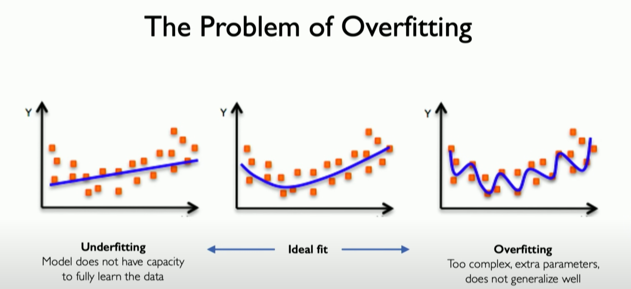
We need to give a brief introduction to overfitting, which can be represented by the far right coordinate graph in the above image.
Definition of Overfitting:
- Overfitting occurs during neural network optimization, especially when using stochastic gradient descent. The essence of overfitting is that the model starts to represent the training data rather than the test data excessively. This means that the model performs very well on the training data but poorly on unseen data.
Core Issue of Overfitting:
- The core issue of overfitting is that the model captures noise and irrelevant features in the training data instead of the true patterns of the underlying data generation process. This results in reduced generalization ability of the model on new data.
Impact of Overfitting:
- Neural networks, due to their extremely high model complexity, are particularly prone to overfitting. Large models have more parameters and weights, allowing them to learn and memorize specific features of the training data in more detail, but this does not always reflect the general characteristics of real-world data.
Detecting Overfitting:
- Overfitting can usually be detected by comparing the model’s performance on the training set and validation set (or test set). If the model performs significantly better on the training set than the validation set, it is often a sign of overfitting.
Scope of Overfitting:
- The occurrence of overfitting can have a significant impact on the success and practical application of neural networks. A severely overfitted model may perform poorly in practical applications because it cannot adapt to new or changing data.
Overfitting is a critical issue in neural network training, involving the problem of a model performing too well on training data while performing poorly on new data. This is usually because the model is too complex, learning noise and specific details in the training data instead of more general data patterns.
Regularization
During the training of neural networks, regularization is a key technique to prevent the model from becoming too complex and thus avoid overfitting. Since neural network models are typically very large, they are particularly prone to overfitting. Therefore, using regularization techniques to promote model generalization to test data, not just training data, is crucial for the success of neural networks.
Definition of Regularization:
- Regularization is a technique introduced into neural networks that helps the model find a balance between being overly
complex and overly simple. This means the model can perform tasks well even when handling completely new data.
Application of Regularization Techniques:
- In practical applications, regularization techniques are not limited to neural networks but are widely used in various machine learning models. For example, a common regularization technique is dropout and early stopping, which stops training at a certain point to prevent overfitting. This point is usually determined when performance on the validation set no longer improves.
Overall, regularization is an important technique to prevent overfitting in machine learning and deep learning models. By introducing some form of constraint or modification, regularization helps the model maintain some generalization ability while learning the data, thus performing well on unseen data.
Dropout
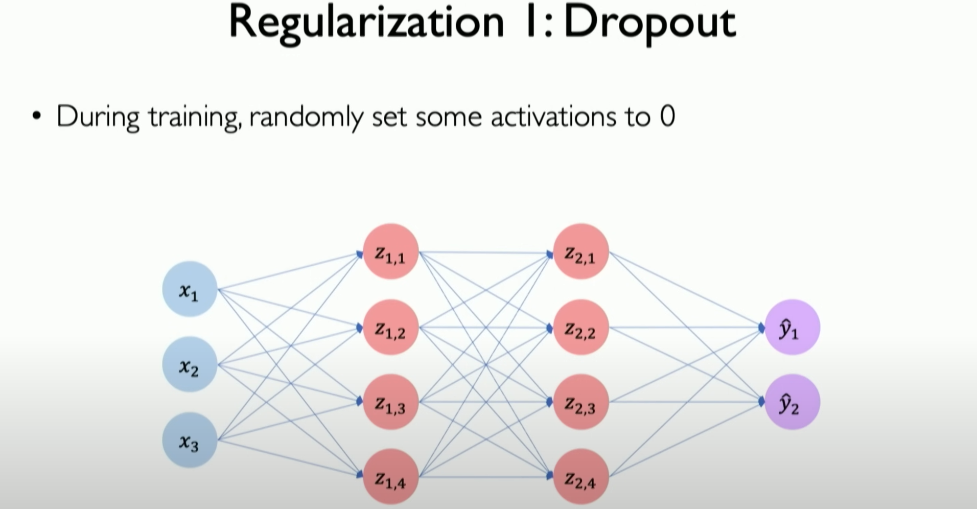
The concept of dropout is very simple: randomly select some subsets of neurons in the neural network during training and try to prune them with some random probability:
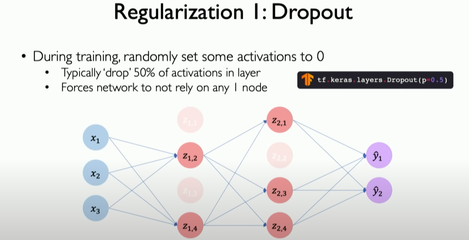
The above image is a simple example. We randomly select a subset of neurons with a 50% probability, randomly turning them off or on in different iterations of training. This behavior mainly forces the model to expose different sets of models internally in each iteration, requiring it to learn how to build internal paths to handle the same information. It cannot rely on what it learned in previous iterations, thus forcing it to capture some deeper meaning in the neural network paths. This approach has two major implications:
- It reduces the capacity of the neural network by approximately 50% in this example.
- It makes the neural network easier to train because the number of weights it has to train is reduced, making the training process faster.
The detailed content of the “Dropout” section includes:
- Concept of Dropout:
- Dropout is one of the most popular regularization techniques in deep learning. The basic idea is to randomly select a portion of neurons from the neural network during training and temporarily remove them from the network.
- Execution of Dropout:
- In each training iteration, randomly select a portion of neurons (e.g., each neuron has a 50% probability of being removed) and ignore their contributions in this iteration. This means these neurons are not active in the forward propagation and backpropagation processes.
- Purpose of Dropout:
- Dropout prevents the network from overfitting to the training data by ensuring that it cannot rely on any single neuron (because they might be randomly removed). Therefore, the network must learn more robust feature representations.
- Effect of Dropout:
- This method effectively reduces complex co-adaptations, where multiple neurons collectively memorize specific features of the training data. The result is a more generalized model with better predictive power on new data.
- Application of Dropout:
- Dropout is typically used in fully connected layers but can also be applied to convolutional layers. It is a simple and effective method that can significantly improve the generalization ability of many deep learning models.
Overall, Dropout is an effective regularization technique that increases the generalization ability and robustness of a model by randomly “shutting down” parts of a neural network during training. This method helps neural networks reduce overfitting to training samples, thus improving performance on new data.
Early Stopping
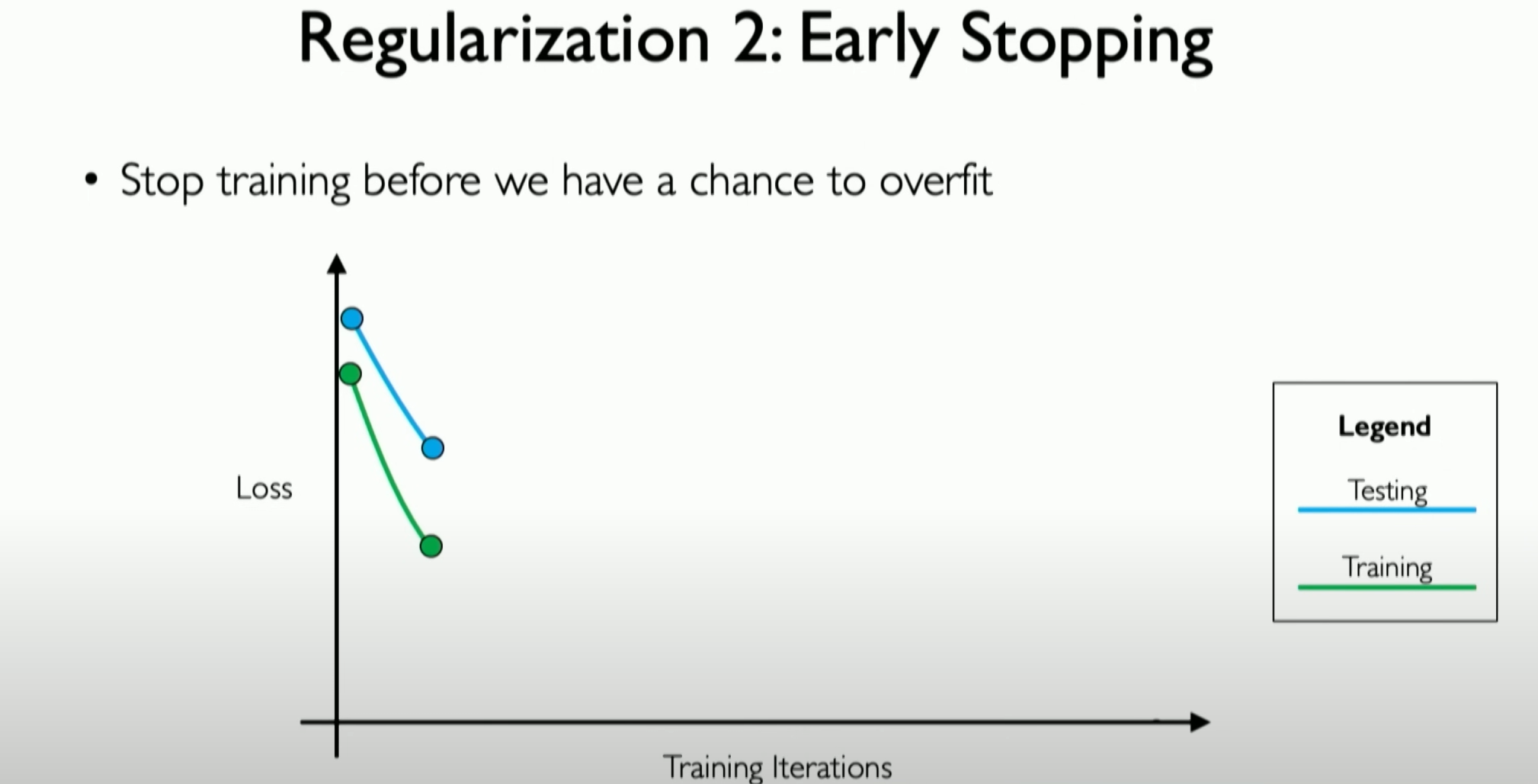
Early stopping is also a regularization technique. Since we know that the essence of overfitting is our model starting to represent the features of the training dataset without generalizing to the test dataset, this is the core of overfitting. In early stopping, we use the validation dataset as a proxy for unseen data to monitor how our network learns this unseen data.
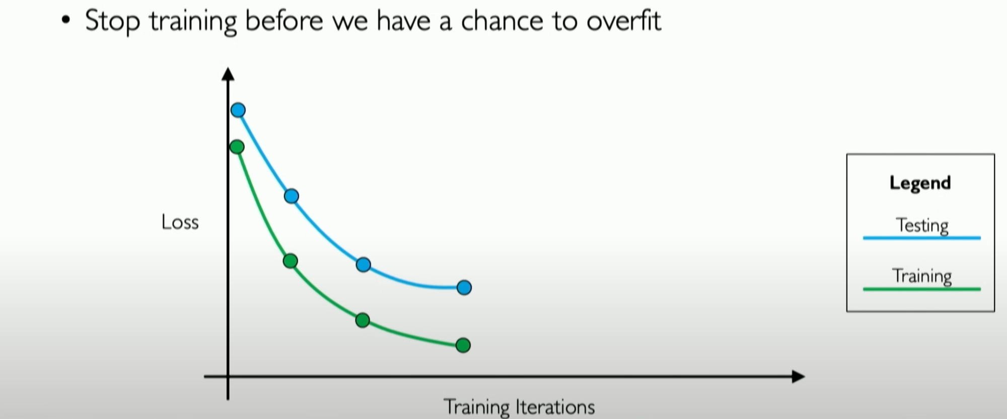
During training, we can see that the losses for both training and validation data decrease, but there will be a point where the validation loss stabilizes and starts to increase. That point is where our neural network starts overfitting the training data.
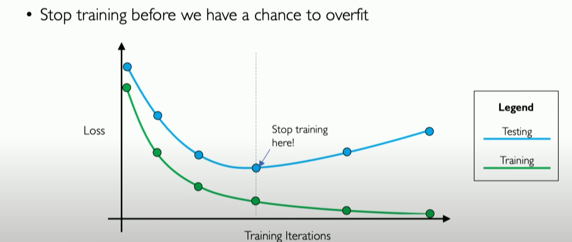
So, the essence of early stopping is to detect the presence of this point and stop training in time because stopping before or after this point will affect the model’s performance.
Summary
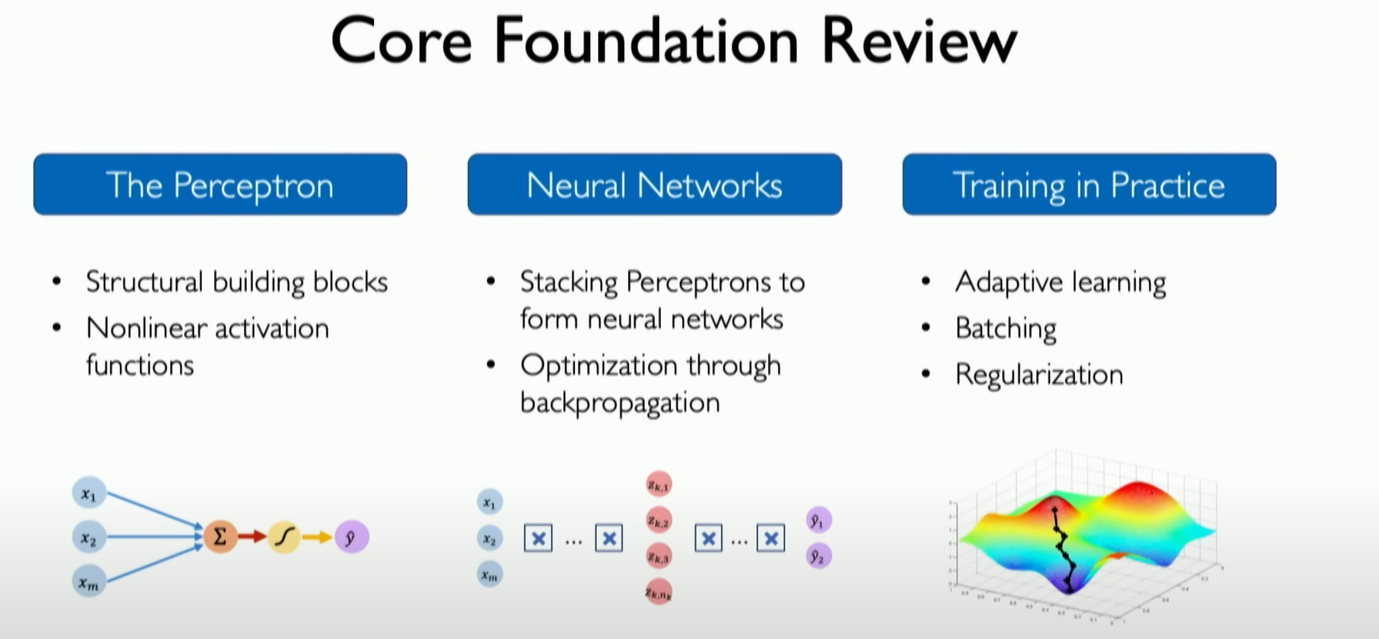
Let’s briefly summarize all the above content. We have learned all the basic building blocks of neural networks, namely single neurons and perceptrons. We have built them into larger neural networks and then from neural networks and deep neural networks. We have learned how to train them and apply them to datasets through backpropagation, and we have learned some techniques and algorithms for end-to-end optimization of these systems.
What Computer “See”
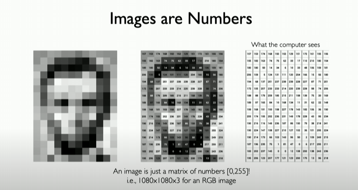
Every image is composed of pixels, and each pixel is a string of numbers. This applies to grayscale images (each pixel is composed of only one number). Additionally, we consider color images (each pixel is composed of three numbers), known as RGB images (Red, Green, Blue). In this way, you can regard a color image as a three-dimensional matrix, composed of three two-dimensional matrices stacked together to form the entire image.
CN
Introduce
首先,我们得知道深度学习可以被用来做什么
诸如:
生成人脸
生成完整的合成环境(full synthetic environments),例如用于训练自动驾驶汽车的道路环境————Vista
根据提示词生成内容(English),甚至可以生成现实数据集中从来都不会出现的图片,例如一个在太空骑马的宇航员(A photo of an astronaut riding a horse)
根据提示词生成图像或视频
根据提示词检索已有的信息,并作出回复
构建生成软件的软件
Deep Learning 在人工智能中的位置
Deep Learning 是 Machine Learning 的一个自己,它明确关注于所谓的神经网络,以及我们该如何构建可以提取数据中特征的神经网络
Why deep learning?
从传统机器学习到深度学习的演变
传统的机器学习算法通常会在数据中定义一组特征,这些特征往往是基于领域知识手工设计的。而深度学习则允许机器自动提取和发现数据中的核心模式,超越了人类定义特征的限制。这使得深度学习算法能够直接从数据中学习更高级别的特征,例如通过识别图像中的边缘、角和曲线来检测脸部等对象。
深度学习模型通过识别图像中的边缘、角和曲线来检测脸部等对象的过程,涉及以下几个主要步骤:
输入图像处理:首先,图像作为输入数据被传送到神经网络。这些图像可能经过预处理,比如缩放、裁剪或归一化,以便于网络处理。提取低级特征:网络的初始层(通常是卷积层)开始处理图像,检测基本的视觉特征,如边缘和线条。这些层通过应用不同的滤波器(或称为卷积核)来识别图像中的低级特征,如水平或垂直边缘。组合中级特征:随着信息在网络层间的传递,后续层会将这些基本特征组合成更复杂的形状和模式。例如,结合直线和曲线可以形成角和其他几何形状。高级特征识别:更深的网络层识别更高级别的特征,如眼睛、鼻子和耳朵。这些特征的识别是基于前面层次识别的边缘和形状。脸部检测:在网络的最后阶段,它会将所有检测到的特征综合起来,以识别整个脸部。这通常涉及到复杂的模式识别,其中神经网络必须从之前的层中学习到的特征中“理解”什么样的组合最有可能表示一个脸部。输出和优化:最终,网络会输出其对图像中是否存在脸部的判断。在训练过程中,这个输出会与实际标签(即图像中是否真的有脸部)进行比较,并根据差异调整网络参数,以提高其在未来识别脸部的准确性。
整个过程是一种分层学习过程,神经网络通过逐层构建从低级到高级的特征来实现复杂任务。这种能力使得深度学习在图像识别和其他领域非常强大。
Why Now?
过去十年在深度学习方面取得了重大进步,这得益于几个关键因素:
大数据的普及:我们处于大数据时代,为深度学习模型提供了前所未有的大量数据,这对它们的性能至关重要。大规模并行化和计算能力:深度学习算法具有高度的并行性,得益于硬件方面的显著进步,使得训练大规模算法和技术成为可能,这在以前是不可行的。开源工具和软件平台:像TensorFlow这样的开源工具和软件平台的出现,使得训练和编码神经网络比以往任何时候都更加容易和可访问。这促进了深度学习领域的更广泛应用和发展。
The perceptron
首先,我们需要知道,在神经网络中,单个神经元(a single neuron)称为感知器(perceptron),我会用一张图来简单说明:
感知器(Perceptron)部分的详细细节如下:
感知器定义:感知器是神经网络中的一个基本单元,相当于单个神经元。它是深度学习中非常基础且简单的概念,主要用于理解神经网络如何工作和传播信息。信息传播:感知器工作的核心是信息的前向传播( forward propagation of information)。这个过程分为三个步骤:点积(dot product)、偏置(bias)、非线性激活函数(non-linearity)。点积和加权输入:要获得感知器的输出,首先需要计算输入与其相应权重的乘积。例如上图,如果感知器有三个输入X1、X2和X3,那么它们分别与各自的权重W1、W2和X3相乘。这些乘积结果被累加以形成一个单一的数值。偏置项:在计算所有输入与权重的乘积之后,还需要添加一个偏置项(通常表示为w0)。偏置项是一个标量权重,可以视为一个恒为1的输入所对应的权重。这一步骤在感知器的运算中至关重要,但有时会被忽略或简化。非线性激活函数:最后,将点积和偏置项的总和通过一个非线性激活函数处理,从而产生感知器的最终输出。这个输出通常表示为Y。非线性激活函数的作用是引入非线性特性,使得网络能够学习并模拟复杂的数据模式和关系。
感知器是神经网络中最基本的构建块之一,其工作原理涉及输入的加权求和、偏置的添加以及非线性激活,这些步骤共同定义了信息在神经网络中的前向传播过程。
Why use non-linearity?
我想,对于非线性激活函数,我们有很多可以讲的东西:非线性激活函数在神经网络中起着至关重要的作用。它们的主要目的是为网络添加非线性特性,这使得网络能够学习和模拟复杂的数据模式和关系。以下是对关于非线性激活函数的进一步解释:
为什么需要非线性:神经网络旨在模拟复杂的、非线性的现实世界数据模式。如果没有非线性激活函数,无论网络有多少层,它本质上都只能执行线性变换,这限制了其表达和学习复杂模式的能力。
如上图,我们无法在线性条件下仅用一条线就完成上面的红绿分离,但是在非线性条件下可以很轻松的处理它。
非线性激活函数允许神经网络建立更复杂的决策边界(Decision Boundary),因此可以处理更复杂的任务,如图像和语音识别。
常见的非线性激活函数:Sigmoid或逻辑函数:这是一种将任意值映射到(0,1)区间的函数,形式为
。它常用于输出层进行二分类。 Tanh(双曲正切)函数:将输入值映射到(-1,1)区间,形式为
。它比Sigmoid函数的输出范围更广,通常有更好的训练性能。 ReLU(Rectified Linear Unit)函数:形式为
。它在正数范围内保持线性,而在负数范围内输出为零。ReLU因其计算简单和训练效果良好而广泛使用。在后面章节我们会详细提到。
激活函数的作用:- 激活函数决定了一个神经元是否应该被激活,即它帮助神经元决定什么信息是重要的,应该进一步传递。
- 它们引入非线性因素,这使得网络能够处理更加复杂和抽象的问题。
激活函数的选择:- 选择特定的激活函数取决于特定的应用和网络架构。例如,对于二元分类问题的输出层,通常使用Sigmoid函数。
- ReLU及其变体(如Leaky ReLU、Parametric ReLU)由于在训练深度网络时的有效性而变得流行。
激活函数的挑战:- 某些激活函数(如Sigmoid和Tanh)可能会导致所谓的“梯度消失”问题,这在训练深度网络时可能导致学习速度变慢。
- ReLU虽然有效,但也有“死亡ReLU”问题,即某些神经元可能永远不会被激活,导致信息丢失。
综上所述,非线性激活函数是神经网络设计的关键组成部分,它们使网络能够学习从简单到复杂的各种数据模式。正确选择和使用激活函数对于构建有效的神经网络模型至关重要。
From perceptrons to neural networks
现在我们回顾之前的内容,重新建立起Perceptron的概念
为了简单起见,我们不画出weight和bias,但它们依然存在,现在的结果是Z,我们将其称为点积(DOT)加上偏差(bias)的结果,这就是我们要传递给非线性函数g的内容,非线性函数g就是关于z的激活函数。
如果我们想要定义和构建一个多层输出神经网络,像上图一样,有两个输出,它依旧是点积(DOT)加上偏差(bias)的结果,两个神经元的对应的两个感知器,都将控制其关联部分的输出。
好了有了上面的数学理解,我们可以将其转换为代码实现,这里我们使用 TensorFlow 和 Keras 来构建我们的密集层(Dense Layer),用于实现自定义的向前传播,也就是我们的perceptron:
1 | import tensorflow as tf |
首先第一部分初始化我们的权重向量(weight Vector),第二部分是我们的偏差向量(bias Vector),接着我们将我们所有的输入和我们的权重进行点积,并加上偏差,再通过一个非线性函数(激活函数)返回结果,这正是call函数所做的。这段代码将运行,这会定义一个完整的神经网络层,然后你就可以像下面这样使用它:
在实际使用Tensorflow时,我们也只需要像上个面这样直接call it即可。
堆叠处理
现在,我们可以正式考虑如何堆叠这些层(layers)来构成一个神经网络
现在,我们仅看一个单层神经网络(Single Layer Neural Network)
让我们简化所有的线条,旨在中间显示这些图标,证明这意味着一切都将完全连接到一起,这覆盖所有的前面提到的数学方程,这并没有增加任何复杂性。好了,在此类型的解决方法上,我们可以接着考虑如何将layer堆叠在彼此之上,这样我们就可以创建所谓的顺序模型(equential models)。
顺序模型(equential models)基本定义了信息的向前传播,不仅是从之前的神经元级别(neuron level),并且扩展到现在的层级别(layer level),每一层都将完全定义,并连接到下一层。下一层的输入将会是前一层所有的输出,在此基础上引入深度神经网络(Deep Neural Network)。
这和之前的没有什么不同,只是这些层经过不断堆叠,通过越来越深入地了解不同层的进展来正确计算最终的输出,最终到达最后一层,即输出层,这就是我们想要输出的最终结果。
Loss functions
首先我们得借助一个例子来引入Loss function的这一概念
我们试着建立一个判断自己是否能通过一门课程的神经网络,他只有两个输入,x1是听的讲座的数量,x2是花在项目上的时间。
我们可以在上图看到在过去几年里学生的数据在这两个输入空间上绘制的二维特征图,来直观的看到两者和最终pass or not的关系。
假设[4,5]这是你的坐标,你想要通过神经网络预判自己是否会pass the class,现在我们抽象出神经网络图:
但我们发现我们经过神经网络的predict后发现通过率仅为0.1,这是为什么?明明我们在数据的二维特征图中,可以看到我们所处的位置在大概率pass的范围内。
原因很简单,这个神经网络没有经过任何数据集的训练,他就像是一张白纸,它不知道passing or failing means。
所以,我们要开始训练它,而这种理解的一部分是我们首先需要告诉neural network它何时犯错了,从数学的角度来讲,我们需要在它犯错时告诉它,它的错误有多大,这样下次他在看到这个数据点时,可以更好地minimize the mistake。在 neural network 中这些 mistakes 被称为 losses(损失)。
具体来讲,我们需要定义一个损失函数(loss function),它将你的prediction和真实的prediction作为输入,告诉你两者的距离有多远,即 how big of a loss there。
我们最终期望的说最小化我们神经网络平均犯下的所有错误
损失函数的定义:- 在神经网络中,损失函数(Loss Function)也可以被称为目标函数(Objective Function)、经验风险(Empirical Risk)、成本函数(Cost Function),这些都是一样的,它用于度量模型预测值与真实值之间的差异。它是一种衡量模型性能的重要工具,帮助指导网络的训练过程。
损失函数的类型:二元分类问题:在处理二元分类问题时,常用的损失函数是softmax交叉熵损失(Softmax Cross-Entropy Loss)。
其他问题:对于其他类型的问题,可能会使用不同的损失函数,如均方误差(Mean Squared Error)用于回归问题。
目标:训练神经网络的目标是找到一组权重(W),使得整个数据集上的损失函数的平均值最小化。
这里的 W 只是一个列表,它只是我们神经网络中所有权重的一组。
损失函数在神经网络训练中扮演了至关重要的角色。它们提供了一种衡量模型性能的方法,并指导模型通过梯度下降或其他优化算法来改进。不同类型的问题可能需要不同的损失函数,选择合适的损失函数对于训练有效的神经网络模型至关重要。
Training and gradient descent
在介绍梯度下降算法之前,我们有必要通过可视化一张简单的 Loss 在三维空间的分布图来,这里仅仅只用两个 weight 作为一组权重来方便可视化,需要注意的是,我们的 loss 就是
起始时,其实是从空间中的随机一个地方开始的,我们可以计算这个特定位置的 loss,最重要的是,实际上我们可以计算 loss 是如何从这个 point 开始变化的,我们可以计算 the gradient of the loss(损失的梯度),因为我们的损失函数是一个连续函数,所以实际上我们可以计算损失函数在权重空间上的导数,梯度告诉我们最高点的方向。
从我们当前所处的位置来看,梯度告诉我们去哪里会增加我们的loss,所以我们实际会向梯度相反的方向迈出一步。
然后不断重复这一过程,直到我们的loss收敛到最小值,现在我们可以将整个梯度下降算法进行总结:
梯度下降(Gradient Descent):- 梯度下降是一种优化算法,用于最小化神经网络的损失函数。
- 过程开始于权重的随机初始化,然后逐步调整权重以减少损失。
- 我们计算 loss 的梯度,并在这个梯度的相反方向更新我们的 W(权重组)。目标是找到使损失最小化的权重组合。
随机梯度下降(Stochastic Gradient Descent):- 在实际应用中,使用随机梯度下降(SGD)而不是传统的梯度下降。SGD在每次迭代中仅使用数据集的一个样本或一小批样本来计算梯度,这加快了计算速度并减少了内存需求。
- 尽管SGD增加了随机性,但它可以更快地收敛,并有助于避免陷入局部最小值。
学习率(Learning Rate):- 学习率是梯度下降中的一个重要参数,决定了权重更新的步长。
- 适当的学习率选择对于快速收敛和避免过度拟合至关重要。
小批量梯度下降(Mini-batch Gradient Descent):- 小批量梯度下降是传统梯度下降和SGD的折中方案,每次迭代使用数据集的一个子集(例如100个数据点)来计算梯度。
- 这种方法在计算效率和梯度估计的准确性之间取得了平衡。
损失函数的计算:- 训练神经网络的目的是最小化损失函数,即模型预测与实际标签之间的差异。
- 不同类型的神经网络和任务可能需要不同的损失函数。
Backpropagation
现在我们必须引入Backpropagation(反向传播)的概念了,因为反向传播算法是计算梯度下降中梯度的关键步骤
反向传播():- 反向传播是计算梯度下降中梯度的关键步骤,它基于链式法则,涉及从输出层向输入层反向传递误差,以有效地更新权重。
- 通过反向传播,每个权重的更新都基于其对最终输出误差的贡献。
我们可以通过链式法则来体现这一过程,它可以确定每个权重,及这些权重的细微变化如果增加或减少,会对我们的损失函数产生多大的影响。这就是Backpropagation algorithm(反向传播算法),这就是训练神经网络的核心。
梯度的计算和传播:- 在单个神经元或感知器级别,首先计算与权重(如W2)相关的导数。
- 然后,这些梯度被反向传播回网络,一直到输入层,以更新相关的权重。
学习率的作用:- 学习率是一个重要参数,决定了在每次迭代中权重更新的步长,也就是在梯度反方向上前进的步长。
- 学习率太高可能导致过度调整,太低则可能导致训练速度过慢。
前向传播与反向传播的关系:
- 前向传播是将信息从输入层传递到输出层的过程。
- 反向传播则是误差从输出层传回输入层的过程,以更新权重。
顺序模型和层级结构:
- 神经网络可以构建为顺序模型,其中每一层都与下一层全连接。
- 在这种结构中,每层的输出成为下一层的输入,形成一个层级的前向传播路径。
反向传播的实现:
- 反向传播算法可以直接实现在各种深度学习框架中,如TensorFlow或PyTorch。
- 它通常包括计算损失函数的梯度,并使用这些梯度来更新网络中的权重。
反向传播的复杂性:
- 虽然理论上反向传播很简单,但在实际操作中可能非常复杂,尤其是在处理大型网络和复杂数据集时。
训练神经网络的过程:
- 反向传播是训练神经网络的一部分,包括将模型应用于数据集,通过反向传播优化权重,以及学习各种技巧和技术以提高训练效果。
在实际训练过程中,神经网络的优化看起来更像下面这样:
Setting the learning rate
学习率的作用:
- 学习率是一个重要参数,决定了在每次迭代中权重更新的步长,也就是在梯度反方向上前进的步长。
- 学习率太高可能导致过度调整,太低则可能导致训练速度过慢。
上面的想要找到最小损失是十分困难的,而上面的
当学习率过大时,很难发生收敛,甚至会发生偏移解决方向的事件
当学习率设置过小也容易发生不在最好出收敛
而我们期望的是它能超越其中的局部最小值,进入搜索空间的合理部分,这样就能收敛到我们所我最关心期望位置。
我们可以想到两者方式来解决这个问题:
一者是不断尝试不同的学习率
更详细的来说,这最终意味着,学习率(即算法信任其观察到的梯度的速度)将取决于几个因素:
- 梯度的大小:在特定位置的梯度大小会影响学习率。如果梯度较大,可能意味着需要较大的学习步长来快速调整权重。
- 学习的速度:学习速度,即网络权重更新的速度,也会影响学习率的选择。快速学习可能需要更高的学习率,以便快速利用大的梯度进行调整。
- 其他选项:在神经网络训练过程中,还可能有其他多种因素和选项影响学习率的设定,如优化算法的选择、网络结构的复杂性等。
学习率的详细细节如下:
学习率过高的影响:- 如果学习率设置得过高,可能导致超调(overshoot),即神经网络从解决方案偏离,梯度可能会爆炸,导致性能恶化。
学习率的挑战性:- 在实践中,确定合适的学习率是一个挑战,因为它会显著影响神经网络的训练和性能。
更智能的学习率设置:- 而不是简单地尝试不同的学习率,可以设计一个能够适应神经网络特性的学习率算法,使其更智能地适应网络的训练过程。
学习率过低的影响:- 设置得太低的学习率会导致学习速度缓慢,甚至可能无法收敛到全局最小值,因为网络可能陷入局部最小值。
自适应学习率算法:- 存在多种自适应学习率算法,这些算法在实践中得到了广泛的研究和应用。Additional details:http://ruder.io/optimizing-gradient-descent/
学习率与梯度下降的更新方程:- 学习率决定了反向传播迭代中梯度下降的步长大小。
提高学习率的可能性:- 通过在批量上平均梯度可以提高梯度的准确性,从而允许提高学习率,并加快学习速度。
学习率与梯度精度的关系:- 梯度的精度提高允许更快地收敛到解决方案,并可能提高学习率的效率。
学习率的实际应用:- 在实际应用中,学习率通常与optimizer(优化器)一起定义,以控制权重的更新速度和方向。
至此,我们可以先停一停,我们可以将前面所提到的所以信息放到一起,合成我们的代码实现
上面的图一共进行了如下步骤:
模型定义:首先,在神经网络的最顶层定义模型。这是讲座开始部分讨论的内容,涉及如何构建和设置神经网络的结构。优化器和学习率:接着,为模型的每个部分定义optimizer(优化器)。优化器与学习率一起被设定,学习率决定了优化损失函数的速度。迭代训练过程:在多个训练循环中,模型会遍历数据集中的所有样本。这个过程涉及观察和理解如何改进神经网络。梯度和网络改进:接下来,基于梯度来改进网络。梯度指示了网络权重需要调整的方向。持续优化:这个过程会反复进行,直到神经网络逐渐收敛到某种解决方案。
Batched gradient descent
我们回顾梯度下降算法的实现过程就可以知道,当数据集很大时,在整个数据集上计算梯度根本不可行,所以我们必须要找一种代替方法,这就要引入Batched gradient descent(批量梯度下降)的概念,即只使用一部分示例数据进行梯度计算,这样虽然会有很大的noisy(噪声),但是计算速度会快得多。
这个公式是小批量梯度下降(Mini-batch Gradient Descent)中用于计算权重(W)的平均梯度的。让我们逐步分析这个公式:
梯度的定义:
表示损失函数 关于权重 的梯度。这个梯度表示损失函数随权重变化的速率,用于指导权重的更新。
小批量的平均梯度:
是在一个小批量中所有样本梯度的平均值。其中 是批量大小,表示小批量中的样本数。 表示第 个样本的损失函数 关于权重 的梯度。
计算过程:
- 首先,对每个样本(
从 1 到 )计算损失函数关于权重的梯度。 - 然后,将这些梯度求和,并除以批量大小
,得到整个批量的平均梯度。
- 首先,对每个样本(
优化和更新:
- 这个平均梯度用于优化过程中更新权重。通过应用这个平均梯度,可以更平滑地调整权重,减少单个样本梯度可能带来的随机性和噪声。
效率和准确性:
- 通过在小批量上计算平均梯度,该方法结合了随机梯度下降的计算效率和全批量梯度下降的准确性。
总的来说,这个公式是小批量梯度下降方法的核心,它通过计算小批量中所有样本梯度的平均值,以有效地更新神经网络中的权重。这种方法在实际应用中既减少了计算负担,又提高了梯度估计的准确性。
批量梯度下降(Batched Gradient Descent)的详细细节如下:
批量数据的概念:- 批量梯度下降涉及将数据分成小批量(mini-batches),每个批量包含数据集中的一小部分数据。
- 这种方法是对梯度下降算法的一种改进,旨在降低计算成本和提高效率。
计算效率和梯度准确性:- 计算整个数据集上的梯度是非常计算密集型的。批量梯度下降通过仅使用数据集的一个小批量来计算梯度,降低了这种计算负担。
- 与单个样本(随机梯度下降)相比,使用小批量可以显著减少随机性,并提高梯度的准确性。
- 通常考虑的批量大小在数十到数百个数据点之间。这样的大小比计算整个数据集的梯度要快得多,同时比基于单个样本的梯度计算更准确。
性能和收敛:- 批量梯度下降平衡了计算效率和梯度估计的准确性,从而在训练过程中提供了更稳定的性能和收敛行为。
- 这种方法允许更快地迭代,并在训练过程中避免了一些梯度下降算法中的极端变化。
实践应用:- 在实际应用中,批量梯度下降是深度学习训练中常见的优化技术,因为它提供了执行速度和梯度估计准确性之间的有效平衡。
总的来说,批量梯度下降是一种在计算效率和梯度估计准确性之间取得平衡的优化方法,适用于大型数据集和复杂的深度学习模型。通过使用数据的小批量,它提高了训练过程中的稳定性和收敛速度。
Regularization: dropout and early stopping
Overfitting
我们需要对overfitting(过拟合)做简短的介绍,它可以由上图最右侧的坐标图表现出来
过拟合的定义:- 过拟合发生在神经网络优化时,特别是使用随机梯度下降法时。过拟合的本质是模型开始过度代表训练数据而不是测试数据。这意味着模型在训练数据上表现得非常好,但在未见过的数据上表现差。
过拟合的核心问题:- 过拟合的核心问题在于,模型捕捉到了训练数据中的噪声和无关特征,而不是底层数据生成过程的真实规律。这导致模型在新数据上的泛化能力受损。
过拟合的影响:- 神经网络由于其极大的模型复杂度,特别容易出现过拟合。大型模型有更多的参数和权重,可以更详细地学习和记忆训练数据的特定特征,但这并不总是反映了真实世界数据的普遍特性。
检测过拟合:- 过拟合通常可以通过比较模型在训练集和验证集(或测试集)上的表现来检测。如果模型在训练集上表现显著优于验证集,这通常是过拟合的一个标志。
过拟合的影响范围:- 过拟合的发生可能对神经网络的成功和实际应用产生重大影响。一个严重过拟合的模型在实际应用中可能表现不佳,因为它无法适应新的或变化的数据。
过拟合是神经网络训练中的一个重要问题,它涉及到模型在训练数据上的性能过于优秀,而在新数据上性能下降的问题。这通常是由于模型过于复杂,学习到了训练数据中的噪声和特定细节,而不是更普遍的数据模式。
Regularization
在训练神经网络的过程中,正则化是一种关键技术,用来防止模型学习过于复杂,从而避免overfitting(过拟合)。由于神经网络模型通常非常大,它们特别容易出现过拟合的问题。因此,使用正则化技术来促使模型泛化到测试数据上,而不仅仅是训练数据上,对神经网络的成功至关重要。
正则化的定义:- 正则化是一种可以引入到神经网络中的技术,它有助于模型在不过于复杂和不过于简单之间找到一个平衡点。这意味着模型能够良好地执行任务,即使在处理全新的数据时也是如此。
正则化技术的应用:- 在实际应用中,正则化技术不仅限于神经网络,而是一种广泛的技术,应用于各种机器学习模型。例如,一种常见的正则化技术是dropout 和 Early Stopping(提前停止),这种方法通过在训练过程中的某个点停止训练来防止过拟合,而这个点通常是在验证集上的性能不再提高时确定的。
总的来说,正则化是一种防止机器学习和深度学习模型过拟合的重要技术。它通过引入一些形式的约束或修改,帮助模型在学习数据的同时保持一定的泛化能力,从而在未见过的数据上也能表现良好。
Dropout
dropout的概念非常简单,即在神经网络训练过程中随机选择该神经网络中的一些神经元子集,并尝试用一些随机概率将它们修剪掉:
上图就是一个很简单的例子,我们随机以50%的概率选择神经元子集,我们在训练的不同迭代中随机关闭或打开它们,这种行为主要是为了强迫模型在每次迭代中,不同的模型的集合都会在内部暴露于一种与上一次迭代时不同的模型,所以它必须学会如何构建内部路径来处理相同的信息,比能切它不能依赖于它在之前几次迭代中学到的信息,因此迫使它在神经网络的路径中捕获一些更深层次的含义。这样的作法有两大意义:
- 它降低了神经网络的容量,在这个例子中大约减少了50%
- 它使神经网络更加易于训练,因为在这种情况下具有的 weights 数量也减少了,所以训练它们实际上也更快
以下是”Dropout” 部分的详细内容包括:
- Dropout的概念:
- Dropout 是深度学习中最流行的正则化技术之一。它的基本思想是在训练过程中随机地从神经网络中选择一部分神经元并将它们临时从网络中移除。
- Dropout的执行方式:
- 在每次训练迭代中,随机选定一部分神经元(例如,每个神经元有50%的概率被移除),并在这次迭代中不考虑它们的贡献。这意味着这些神经元在前向传播和后向传播过程中都不活跃。
- Dropout的目的:
- 通过这种方式,Dropout 防止了网络对训练数据的过度依赖和拟合。因为网络不能依赖于任何单一的神经元(因为它们可能被随机移除),所以网络必须学习更加鲁棒的特征表示。
- Dropout的效果:
- 这种方法有效地减少了复杂的协同适应现象,即多个神经元共同记住训练数据的特定特征。结果是一个更加泛化的模型,对新数据的预测能力更强。
- Dropout的应用:
- Dropout 通常用于全连接层,但也可以用于卷积层。它是一种简单而有效的方法,可以显著提高许多深度学习模型的泛化能力。
总体来说,Dropout 是一种有效的正则化技术,通过在训练过程中随机“关闭”神经网络的一部分,来增加模型的泛化能力和鲁棒性。这种方法能够帮助神经网络减少对训练样本的过度拟合,从而提高在新数据上的性能。
early stopping
early stopping(早停)也是正则化技术中的一种,由于我们知道所谓的 overfitting(过拟合)实质是我们的模型开始表现为训练数据集的特征而没有泛化到测试数据集,这就是过拟合的核心,在 early stopping 的概念中,我们将其作为一种测试数据集(综合测试数据集),我们可以通过它来监控我们的网络是如何学习这部分看不见的数据的。
在训练中,我们可以看到,这两者的 loss 都会减少,但会出现一个 test loss 趋于稳定,并开始增加的点,那个点实际就是我们的神经网络开始过拟合训练数据的点。
所以 early stopping 的实质就是,检测出这个点的存在,并及时停止训练,因为在这个 point 之前或之后停止都会影响 model 的性能。
Summary
我们简要的总结一下上面的所有内容,我们已经了解了所有神经网络的基本构建块,即单个神经元和感知器,我们将它们构建成更大的神经网络,然后从它们的神经网络和深度神经网络中,我们了解了该如何训练它们并将它们应用到通过它们反向传播的数据集,并且我们已经学到了一些用于端到端优化的这些系统的技巧和算法。
What Computer “See”
每一张图像,都是由像素组成的,而每一个像素都是一串数字,这适用于灰度图(每个像素仅由一个数字构成),我们另外考虑彩色图像(每个像素由三个数字构成),所以被称为RGB图像(Red、Green、Blue),这样,你可以将彩色图像视为一个三维矩阵,即由三个二维矩阵构成,它们堆叠在一起构成了整张图像