Lab1-Part1_TensorFlow
Q7nl1s admin

EN

API

TensorFlowhttps://www.tensorflow.org/api_docs/python/tf

tf.GradientTape | TensorFlow v2.14.0

Keras API Tutorial:Keras | TensorFlow Core

kerashttps://www.tensorflow.org/api_docs/python/tf/keras

tf.keras.Input | TensorFlow v2.0.0

tf.keras.Model | TensorFlow v2.14.0

tf.keras.Sequential | TensorFlow v2.14.0

layershttps://www.tensorflow.org/api_docs/python/tf/keras/layers/

tf.keras.layers.Dense | TensorFlow v2.14.0

perceptron

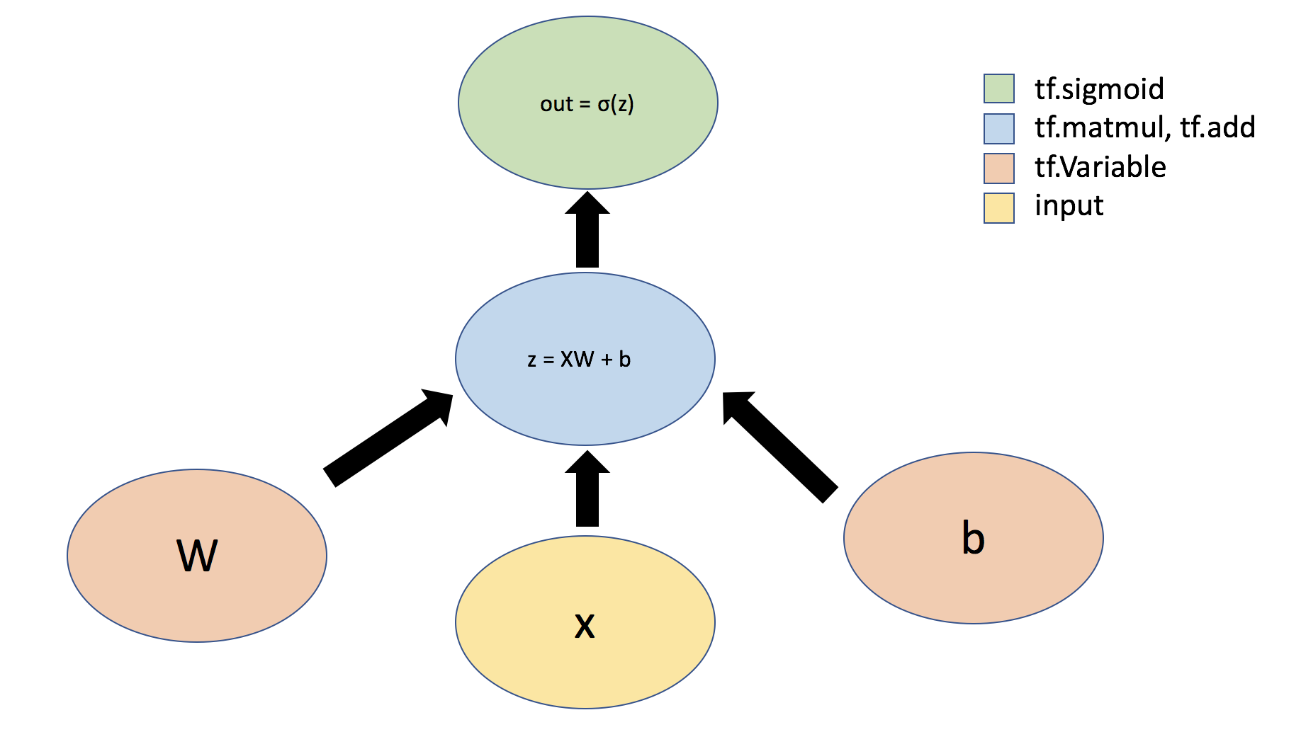
Tensors can flow through an abstract type called Layers — they are the building blocks of neural networks.

Layers implement common neural network operations and are used to update weights, compute losses, and define layer connections.

An example of implementing a perceptron, which is built using a dense layer (also known as a fully connected layer).
alt text

1
2
3
4
5
6
7
8
9
10
11
12
13
14
15
16
17
18
19
20
21
22
23
24
25
26
27
28
29
30
31
32
33
34
35
36
### Defining a network Layer ###

# n_output_nodes: number of output nodes
# input_shape: shape of the input
# x: input to the layer

class OurDenseLayer(tf.keras.layers.Layer):
def __init__(self, n_output_nodes):
super(OurDenseLayer, self).__init__()
self.n_output_nodes = n_output_nodes

def build(self, input_shape):
d = int(input_shape[-1])
# Define and initialize parameters: a weight matrix W and bias b
# Note that parameter initialization is random!
self.W = self.add_weight("weight", shape=[d, self.n_output_nodes]) # note the dimensionality
self.b = self.add_weight("bias", shape=[1, self.n_output_nodes]) # note the dimensionality

def call(self, x):
'''TODO: define the operation for z (hint: use tf.matmul)'''
z = tf.matmul(x, self.W) + self.b # TODO

'''TODO: define the operation for out (hint: use tf.sigmoid)'''
y = tf.sigmoid(z) # TODO
return y

# Since layer parameters are initialized randomly, we will set a random seed for reproducibility
tf.random.set_seed(1)
layer = OurDenseLayer(3) # Create an instance of OurDenseLayer with 3 output nodes
layer.build((1, 2)) # Initialize the weights and biases with input shape (1, 2)
x_input = tf.constant([[1, 2.]], shape=(1, 2)) # Create a constant input tensor with shape (1, 2)
y = layer.call(x_input)

# Test the output!
print(y.numpy())
mdl.lab1.test_custom_dense_layer_output(y)
  • The initialization of self.W weights is usually random, which helps to break symmetry and start the learning process. TensorFlow provides various initialization methods, such as random normal distribution and uniform distribution. During the training of the network, this weight matrix will be continuously updated according to the backpropagation algorithm and optimizer to minimize the loss function and improve the model’s performance.
  • Unlike the initialization of the weight matrix, the self.bias bias vector is typically initialized to zero or near-zero small values. This is because the main role of the bias is to provide a learnable offset rather than to break symmetry (which is the primary purpose of weight initialization). Initializing the bias to zero is a common practice as it does not affect the initial state of the network. As training progresses, the bias will be adjusted based on gradient descent and backpropagation algorithms to help the model better fit the data.

Building Neural Networks with the Sequential API

TensorFlow has predefined many commonly used Layers in neural networks, such as the Dense layer. Now, instead of using a single Layer to define our simple neural network, we will use the Sequential model and a Dense layer from Keras to define our network. The Sequential API allows you to easily create neural networks by stacking layers like building blocks.

1
2
3
4
5
6
7
8
9
10
11
12
13
14
15
16
17
18
19
20
21
22
23
24
25
### Defining a neural network using the Sequential API ###

# Import relevant packages
from tensorflow.keras import Sequential
from tensorflow.keras.layers import Dense

# Define the number of outputs
n_output_nodes = 3

# First define the model
model = Sequential()

'''TODO: Define a dense (fully connected) layer to compute z'''
# Remember: dense layers are defined by the parameters W and b!
# You can read more about the initialization of W and b in the TF documentation :)
# https://www.tensorflow.org/api_docs/python/tf/keras/layers/Dense?version=stable
dense_layer = Dense(
n_output_nodes, # Use n_output_nodes as the number of units in the layer
activation="sigmoid",
use_bias=True,
bias_initializer='zeros'
) # TODO

# Add the dense layer to the model
model.add(dense_layer)

Test

1
2
3
4
5
6
# Test model with example input
x_input = tf.constant([[1, 2.]], shape=(1, 2))

'''TODO: feed input into the model and predict the output!'''
model_output = model.call(x_input) # TODO
print(model_output)

Output: tf.Tensor([[0.7611146 0.7311695 0.8857081]], shape=(1, 3), dtype=float32)

Defining Neural Networks by Subclassing the Model Class

Besides using the Sequential API to define models, we can also define neural networks by subclassing the Model class. This class groups layers together to enable training and inference. The Model class defines what we refer to as a “model” or “network.” By subclassing, we can create a class for our model and use the call function to define the forward pass of the network. Subclassing provides the flexibility to define custom layers, custom training loops, custom activation functions, and custom models.

1
2
3
4
5
6
7
8
9
10
11
12
13
14
15
16
17
18
19
20
21
### Defining a model using subclassing ###

from tensorflow.keras import Model
from tensorflow.keras.layers import Dense

class SubclassModel(tf.keras.Model):

# In __init__, we define the Model's layers
def __init__(self, n_output_nodes):
super(SubclassModel, self).__init__()
'''TODO: Our model consists of a single Dense layer. Define this layer.'''
self.dense_layer = Dense(
n_output_nodes, # Use n_output_nodes as the number of units in the layer
activation="sigmoid",
use_bias=True,
bias_initializer='zeros'
) # TODO: Dense Layer

# In the call function, we define the Model's forward pass.
def call(self, inputs):
return self.dense_layer(inputs)

Test

1
2
3
4
5
6
n_output_nodes = 3
model = SubclassModel(n_output_nodes)

x_input = tf.constant([[1, 2.]], shape=(1, 2))

print(model.call(x_input))

Output: tf.Tensor([[0.7440547 0.22250177 0.33796322]], shape=(1, 3), dtype=float32)

Subclassing provides the flexibility to define custom layers, custom training loops, custom activation functions, and custom models

For example, defining a boolean parameter isidentity to control whether the input is simply outputted without any alteration.

1
2
3
4
5
6
7
8
9
10
11
12
13
14
15
16
17
18
19
20
21
22
23
24
### Defining a model using subclassing and specifying custom behavior ###

from tensorflow.keras import Model
from tensorflow.keras.layers import Dense

class IdentityModel(tf.keras.Model):

# As before, in __init__ we define the Model's layers
# Since our desired behavior involves the forward pass, this part is unchanged
def __init__(self, n_output_nodes):
super(IdentityModel, self).__init__()
self.dense_layer = tf.keras.layers.Dense(n_output_nodes, activation='sigmoid')

'''TODO: Implement the behavior where the network outputs the input, unchanged,


under control of the isidentity argument.'''
def call(self, inputs, isidentity=False):
x = self.dense_layer(inputs)
# When isidentity is True, return the original input; otherwise, return the output of the layer
if isidentity:
return inputs
return x
'''TODO: Implement identity behavior'''

Test

1
2
3
4
5
6
7
8
9
n_output_nodes = 3
model = IdentityModel(n_output_nodes)

x_input = tf.constant([[1, 2.]], shape=(1, 2))
'''TODO: pass the input into the model and call with and without the input identity option.'''
out_activate = model.call(x_input, False) # TODO
out_identity = model.call(x_input, True) # TODO

print("Network output with activation: {}; network identity output: {}".format(out_activate.numpy(), out_identity.numpy()))

Output: Network output with activation: [[0.24258928 0.8098861 0.9044685 ]]; network identity output: [[1. 2.]]

Differentiation and Stochastic Gradient Descent (SGD)

Automatic differentiation is one of the most important parts of TensorFlow and is the basis for training using backpropagation. We will use TensorFlow’s GradientTape tf.GradientTape to track operations so we can later compute gradients.

When performing a forward pass through the network, all forward-pass operations are recorded onto a “tape.” To compute the gradients, the tape is then played backwards. By default, the tape is discarded after it is played backwards; this means a particular tf.GradientTape can only compute gradients once, and subsequent calls will throw runtime errors. However, we can create a persistent gradient tape to compute multiple gradients for the same computation.

We define a simple function ( y = x^2 ) and compute the gradient:

1
2
3
4
5
6
7
8
9
10
11
12
13
14
### Gradient computation with GradientTape ###

# y = x^2
# Example: x = 3.0
x = tf.Variable(3.0)

# Initiate the gradient tape
with tf.GradientTape() as tape:
# Define the function
y = x * x
# Access the gradient -- derivative of y with respect to x
dy_dx = tape.gradient(y, x)

assert dy_dx.numpy() == 6.0

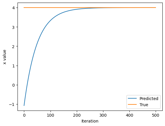
In training neural networks, we use differentiation and Stochastic Gradient Descent (SGD) to optimize the loss function. Now that we understand how to use GradientTape to compute and access derivatives, we will look at an example where we use automatic differentiation and SGD to find the minimum of ( L=(x-x_f)^2 ). Here, ( x_f ) is a variable representing the desired value we are trying to optimize for; ( L ) represents the loss we are working to minimize. While we can obviously solve this problem analytically (( x_{min}=x_f )), considering how to solve it using GradientTape lays a good foundation for our future experiments where we will use gradient descent to optimize neural network loss.

1
2
3
4
5
6
7
8
9
10
11
12
13
14
15
16
17
18
19
20
21
22
23
24
25
26
27
28
29
30
### Function minimization with automatic differentiation and SGD ###

# Initialize a random value for our initial x
x = tf.Variable([tf.random.normal([1])])
print("Initializing x={}".format(x.numpy()))

learning_rate = 1e-2 # learning rate for SGD
history = []
# Define the target value
x_f = 4

# We will run SGD for a number of iterations. At each iteration, we compute the loss,
# compute the derivative of the loss with respect to x, and perform the SGD update.
for i in range(500):
with tf.GradientTape() as tape:
'''TODO: define the loss as described above'''
loss = (x-x_f)**2 # TODO

# loss minimization using gradient tape
grad = tape.gradient(loss, x) # compute the derivative of the loss with respect to x
new_x = x - learning_rate*grad # sgd update
x.assign(new_x) # update the value of x
history.append(x.numpy()[0])

# Plot the evolution of x as we optimize towards x_f!
plt.plot(history)
plt.plot([0, 500],[x_f,x_f])
plt.legend(('Predicted', 'True'))
plt.xlabel('Iteration')
plt.ylabel('x value')

Output:

Initializing x=[[-1.1771784]]
Text(0, 0.5, 'x value')

download

GradientTape provides a highly flexible automatic differentiation framework. To backpropagate errors through a neural network, we track the forward-pass operations on tape, use this information to determine gradients, and then use these gradients to optimize using SGD.

Issue

==UsageError: Line magic function %tensorflow_version not found.==

Jupyter Notebook comes with a set of magic functions, but %tensorflow_version is not one of them.

The magic command

1
%tensorflow_version X.X

is only available in Google Colab notebooks, not Jupyter notebooks.

Instead, you need to use the command line to install a specific version, such as:

1
pip install tensorflow==1.15.0

Or within the Jupyter notebook itself:

1
2
3
import sys 
!{sys.executable} -m pip install tensorflow==1.15.0
# !{sys.executable} -m pip install --user tensorflow==1.15.0. # you may need '--user' based on your environment

==Difference between tf.matmul and tf.multiply==

In neural networks, tf.matmul and tf.multiply serve very different purposes:

Take ( y = \sigma(Wx + b) ) as an example:

  1. tf.matmul: This function is used for matrix multiplication. In the dense layer of a neural network, the relationship between input x (a vector or a batch of vectors) and weights W (a matrix) is typically defined through matrix multiplication. The operation tf.matmul(x, W) involves multiplying each element of x with the corresponding element in W and summing over each row to produce the output. This is a standard linear transformation operation and is one of the fundamental building blocks in neural networks.
  2. tf.multiply: This function performs element-wise multiplication (also known as the Hadamard product or pointwise multiplication). It operates on two tensors of the same shape and multiplies corresponding elements. This means that the input tensor and the weight tensor must have the same shape, which is not common in standard dense layers.

In the OurDenseLayer class, using tf.matmul is the correct choice because we need to perform an operation that multiplies the input tensor x (shape [batch_size, d]) with the weight matrix W (shape [d, n_output_nodes]). This matrix multiplication is the standard method for constructing neural network layers, effectively mapping input data to a new (often higher-dimensional) space, providing inputs for subsequent non-linear activation functions like sigmoid.

In summary, tf.matmul is used for matrix multiplication, which is key for implementing linear transformations in neural network layers, while tf.multiply is used for element-wise multiplication, typically for different operations (e.g., applying pointwise activation functions in certain special types of layers). When building standard dense layers, you should use tf.matmul.


CN

Colaboratory 链接:“Part1_TensorFlow.ipynb”的副本 - Colaboratory (google.com)

API

TensorFlowhttps://www.tensorflow.org/api_docs/python/tf

tf.GradientTape | TensorFlow v2.14.0

Keras API教程:Keras | TensorFlow Core

kerashttps://www.tensorflow.org/api_docs/python/tf/keras

tf.keras.Input | TensorFlow v2.0.0

tf.keras.Model | TensorFlow v2.14.0

tf.keras.Sequential | TensorFlow v2.14.0

layershttps://www.tensorflow.org/api_docs/python/tf/keras/layers/

tf.keras.layers.Dense | TensorFlow v2.14.0

perceptron

张量可以通过被称为Layers的抽象类型进行流动 —— 它们是神经网络的构建块。

Layers实现了常见的神经网络操作,并用于更新权重、计算损失以及定义层间连接。

实现一个感知器的例子,它由一个 dense layer(密集层定义,也叫全连接层)来构建的

alt text

1
2
3
4
5
6
7
8
9
10
11
12
13
14
15
16
17
18
19
20
21
22
23
24
25
26
27
28
29
30
31
32
33
34
35
36
37
### Defining a network Layer ###

# n_output_nodes: number of output nodes
# input_shape: shape of the input
# x: input to the layer


class OurDenseLayer(tf.keras.layers.Layer):
def __init__(self, n_output_nodes):
super(OurDenseLayer, self).__init__()
self.n_output_nodes = n_output_nodes

def build(self, input_shape):
d = int(input_shape[-1])
# Define and initialize parameters: a weight matrix W and bias b
# Note that parameter initialization is random!
self.W = self.add_weight("weight", shape=[d, self.n_output_nodes]) # note the dimensionality
self.b = self.add_weight("bias", shape=[1, self.n_output_nodes]) # note the dimensionality

def call(self, x):
'''TODO: define the operation for z (hint: use tf.matmul)'''
z = tf.matmul(x,self.W) + self.b# TODO

'''TODO: define the operation for out (hint: use tf.sigmoid)'''
y = tf.sigmoid(z)# TODO
return y

# Since layer parameters are initialized randomly, we will set a random seed for reproducibility
tf.random.set_seed(1)
layer = OurDenseLayer(3) # 创建 OurDenseLayer 的一个实例,指定输出节点数为 3
layer.build((1,2)) # 调用 build 方法初始化层的权重和偏置,输入形状为 (1, 2)
x_input = tf.constant([[1,2.]], shape=(1,2)) # 创建一个形状为 (1, 2) 的常量输入张量
y = layer.call(x_input)

# test the output!
print(y.numpy())
mdl.lab1.test_custom_dense_layer_output(y)
  • 上面的 self.W 权重的初始化通常是随机的,这有助于打破对称性并开始学习过程。TensorFlow 提供了多种初始化方法,如随机正态分布、均匀分布等。在网络的训练过程中,这个权重矩阵会根据反向传播算法和优化器不断更新,以最小化损失函数,从而提高模型的性能。
  • 与权重矩阵的初始化略有不同,self.bais 偏置向量通常是以零或者接近零的小数进行初始化。这是因为偏置的主要作用是提供一个可学习的偏移量,而不是打破对称性(这是权重初始化的主要目的)。初始化偏置为零是一个常用的做法,因为这样做不会影响网络的初始状态。随着训练的进行,偏置会根据梯度下降和反向传播算法进行调整,以帮助模型更好地拟合数据。

通过 Sequential API 来构建神经网络

TensorFlow已经定义了许多在神经网络中常用的Layers,例如Dense层。现在,我们不是使用单个Layer来定义我们的简单神经网络,而是使用Keras中的Sequential模型和一个Dense层来定义我们的网络。通过Sequential API,你可以通过像搭积木一样堆叠层来轻松创建神经网络。

1
2
3
4
5
6
7
8
9
10
11
12
13
14
15
16
17
18
19
20
21
22
23
24
25
26
### Defining a neural network using the Sequential API ###

# Import relevant packages
from tensorflow.keras import Sequential
from tensorflow.keras.layers import Dense

# Define the number of outputs
n_output_nodes = 3

# First define the model
model = Sequential()

'''TODO: Define a dense (fully connected) layer to compute z'''
# Remember: dense layers are defined by the parameters W and b!
# You can read more about the initialization of W and b in the TF documentation :)
# https://www.tensorflow.org/api_docs/python/tf/keras/layers/Dense?version=stable
dense_layer = Dense(
n_output_nodes, # 使用 n_output_nodes 作为层的单元数
activation="sigmoid",
use_bias=True,
bias_initializer='zeros'
)# TODO

# Add the dense layer to the model
model.add(dense_layer)

test

1
2
3
4
5
6
# Test model with example input
x_input = tf.constant([[1,2.]], shape=(1,2))

'''TODO: feed input into the model and predict the output!'''
model_output = model.call(x_input)# TODO
print(model_output)

output:tf.Tensor([[0.7611146 0.7311695 0.8857081]], shape=(1, 3), dtype=float32)

直接子类化Model类来定义神经网络

除了使用Sequential API定义模型外,我们还可以通过直接子类化Model类来定义神经网络,这个类将层组合在一起,使模型训练和推理成为可能。Model类定义了我们所说的“模型”或“网络”。使用子类化,我们可以为我们的模型创建一个类,并使用call函数定义网络的前向传递。子类化提供了定义自定义层、自定义训练循环、自定义激活函数和自定义模型的灵活性。

1
2
3
4
5
6
7
8
9
10
11
12
13
14
15
16
17
18
19
20
21
### Defining a model using subclassing ###

from tensorflow.keras import Model
from tensorflow.keras.layers import Dense

class SubclassModel(tf.keras.Model):

# In __init__, we define the Model's layers
def __init__(self, n_output_nodes):
super(SubclassModel, self).__init__()
'''TODO: Our model consists of a single Dense layer. Define this layer.'''
self.dense_layer = Dense(
n_output_nodes, # 使用 n_output_nodes 作为层的单元数
activation="sigmoid",
use_bias=True,
bias_initializer='zeros'
) # TODO: Dense Layer

# In the call function, we define the Model's forward pass.
def call(self, inputs):
return self.dense_layer(inputs)

test

1
2
3
4
5
6
n_output_nodes = 3
model = SubclassModel(n_output_nodes)

x_input = tf.constant([[1,2.]], shape=(1,2))

print(model.call(x_input))

output:tf.Tensor([[0.7440547 0.22250177 0.33796322]], shape=(1, 3), dtype=float32)

子类化提供了定义自定义层、自定义训练循环、自定义激活函数和自定义模型的灵活性

比如定义了一个布尔参数isidentity来控制定义了一个布尔参数isidentity来控制简单地输出输入,不进行任何干扰

1
2
3
4
5
6
7
8
9
10
11
12
13
14
15
16
17
18
19
20
21
22
### Defining a model using subclassing and specifying custom behavior ###

from tensorflow.keras import Model
from tensorflow.keras.layers import Dense

class IdentityModel(tf.keras.Model):

# As before, in __init__ we define the Model's layers
# Since our desired behavior involves the forward pass, this part is unchanged
def __init__(self, n_output_nodes):
super(IdentityModel, self).__init__()
self.dense_layer = tf.keras.layers.Dense(n_output_nodes, activation='sigmoid')

'''TODO: Implement the behavior where the network outputs the input, unchanged,
under control of the isidentity argument.'''
def call(self, inputs, isidentity=False):
x = self.dense_layer(inputs)
# 当 isidentity 为 True 时,返回原始输入,否则返回层的输出
if isidentity:
return inputs
return x
'''TODO: Implement identity behavior'''

test

1
2
3
4
5
6
7
8
9
n_output_nodes = 3
model = IdentityModel(n_output_nodes)

x_input = tf.constant([[1,2.]], shape=(1,2))
'''TODO: pass the input into the model and call with and without the input identity option.'''
out_activate = model.call(x_input,False)# TODO
out_identity = model.call(x_input,True)# TODO

print("Network output with activation: {}; network identity output: {}".format(out_activate.numpy(), out_identity.numpy()))

output:Network output with activation: [[0.24258928 0.8098861 0.9044685 ]]; network identity output: [[1. 2.]]

微分和随机梯度下降(SGD)

自动微分是TensorFlow最重要的部分之一,也是使用反向传播训练的基础。我们将使用 TensorFlow 的 GradientTape tf.GradientTape来跟踪操作,以便稍后计算梯度。

当通过网络进行前向传递时,所有前向传递操作都会被记录到一个“磁带”上;然后,为了计算梯度,磁带被反向播放。默认情况下,磁带在反向播放后会被丢弃;这意味着一个特定的tf.GradientTape只能计算一次梯度,随后的调用会抛出运行时错误。然而,我们可以通过创建一个persistent的梯度磁带来对同一计算计算多个梯度。

我们定义了一个简单的函数 并计算梯度:

1
2
3
4
5
6
7
8
9
10
11
12
13
14
### Gradient computation with GradientTape ###

# y = x^2
# Example: x = 3.0
x = tf.Variable(3.0)

# Initiate the gradient tape
with tf.GradientTape() as tape:
# Define the function
y = x * x
# Access the gradient -- derivative of y with respect to x
dy_dx = tape.gradient(y, x)

assert dy_dx.numpy() == 6.0

在训练神经网络中,我们使用微分和随机梯度下降(SGD)来优化损失函数。现在我们已经了解了如何使用 GradientTape 来计算和访问导数,我们将看一个例子,其中我们使用自动微分和 SGD 来找到 的最小值。这里的 是一个我们试图优化的期望值的变量; 代表我们正在努力最小化的损失。虽然我们显然可以通过解析方法解决这个问题(),但考虑如何使用 GradientTape 来计算这个问题,为我们未来使用梯度下降优化整个神经网络损失的实验室打下了良好的基础。

1
2
3
4
5
6
7
8
9
10
11
12
13
14
15
16
17
18
19
20
21
22
23
24
25
26
27
28
29
30
### Function minimization with automatic differentiation and SGD ###

# Initialize a random value for our initial x
x = tf.Variable([tf.random.normal([1])])
print("Initializing x={}".format(x.numpy()))

learning_rate = 1e-2 # learning rate for SGD
history = []
# Define the target value
x_f = 4

# We will run SGD for a number of iterations. At each iteration, we compute the loss,
# compute the derivative of the loss with respect to x, and perform the SGD update.
for i in range(500):
with tf.GradientTape() as tape:
'''TODO: define the loss as described above'''
loss = (x-x_f)**2 # TODO

# loss minimization using gradient tape
grad = tape.gradient(loss, x) # compute the derivative of the loss with respect to x
new_x = x - learning_rate*grad # sgd update
x.assign(new_x) # update the value of x
history.append(x.numpy()[0])

# Plot the evolution of x as we optimize towards x_f!
plt.plot(history)
plt.plot([0, 500],[x_f,x_f])
plt.legend(('Predicted', 'True'))
plt.xlabel('Iteration')
plt.ylabel('x value')

output:

Initializing x=[[-1.1771784]]
Text(0, 0.5, ‘x value’)
download

GradientTape提供了一个非常灵活的自动微分框架。为了通过神经网络反向传播误差,我们在磁带上跟踪前向传递的操作,利用这些信息来确定梯度,然后使用这些梯度来使用SGD进行优化。

issue

==UsageError: Line magic function %tensorflow_version not found.==

Jupyter Notebook 附带了一组神奇函数,但 %tensorflow_version 不是其中之一。 magic command

1
%tensorflow_version X.X

只适用于 Google Colab 笔记本,不适用于 Jupyter 笔记本。

而是需要用命令行,安装特定的版本,如:

1
pip install tensorflow==1.15.0

或 Jupyter 笔记本本身:

1
2
3
import sys 
!{sys.executable} -m pip install tensorflow==1.15.0
# !{sys.executable} -m pip install --user tensorflow==1.15.0. # you may need '--user' based on your environment

==tf.matmul和tf.multiply的区别==

在神经网络中,tf.matmultf.multiply 有着非常不同的作用:

为例:

  1. tf.matmul: 这个函数用于执行矩阵乘法。在神经网络的密集层中,输入 x(一个向量或一个批量的向量)和权重 W(一个矩阵)之间的关系通常通过矩阵乘法来定义。tf.matmul(x, W) 的操作是将输入 x 的每个元素与 W 中相应的元素相乘,并对每行求和,从而得到输出。这是标准的线性变换操作,是神经网络中最基本的组成部分之一。
  2. tf.multiply: 这个函数用于执行元素间的乘法(也称为哈达玛积或点对点乘法)。它对两个形状相同的张量进行操作,并将这两个张量中相对应位置的元素相乘。这意味着输入张量和权重张量必须有相同的形状,这在标准的密集层中并不常见。

OurDenseLayer 类中,使用 tf.matmul 是正确的选择,因为我们需要执行的操作是将输入张量 x(形状为 [batch_size, d])和权重矩阵 W(形状为 [d, n_output_nodes])相乘。这种矩阵乘法是构建神经网络层的标准方法,它可以有效地将输入数据映射到新的(通常更高维的)空间,为后续的非线性激活函数(如sigmoid)提供输入。

总结来说,tf.matmul 用于矩阵乘法,它是实现神经网络层中线性变换的关键操作,而 tf.multiply 用于元素间的乘法,通常用于执行不同的操作(例如,在某些特殊类型的层中应用逐元素的激活函数)。在构建标准的密集层时,您应该使用 tf.matmul

 Comments
Comment plugin failed to load
Loading comment plugin
Powered by Hexo & Theme Keep
Unique Visitor Page View