

EN
Textbook link: https://zh-v2.d2l.ai/chapter_preliminaries/ndarray.html
Data Manipulation
There are generally two ways to handle data in deep learning, taking Pytorch as an example
- Python’s NumPy package: only supports CPU computation
- Pytorch’s Tensor: supports GPU accelerated computation
Note, the data we are dealing with, i.e., n-dimensional arrays, are also called tensors.
Getting Started
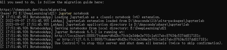
Let’s first enter the jupyter environment
1 | jupyter notebook |
Then find the corresponding chapter’s ipynb file, here it’s data manipulation
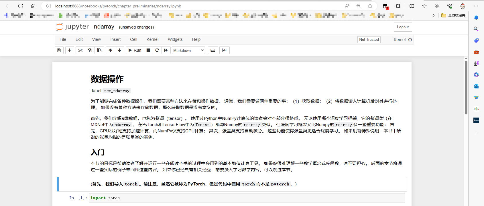
Next, we can debug after importing the torch package


Of course, you can also modify the code for debugging

Here’s a reminder: for better understanding, we can imagine that in a torch.zeros(...) the number of parameters determines the tensor’s dimensions. Taking the above example,
Starting from the right, the first 3 represents a vector of size 3, wrapped in one layer of brackets [].
Next, from the right, the second 4 represents a 2D matrix composed of four 1D vectors, also wrapped in one layer of brackets [].
The third 2 similarly represents a 3D tensor composed of two 2D matrices, again wrapped in one layer of brackets []. It’s quite simple.
Always remember to look from right to left.
1 | torch.arange(12) # Create a vector of 12 integers starting from 0 |
Operators
For any tensors with the same shape, [common standard arithmetic operators (+, -, *, /, and **) can be upgraded to element-wise operations].
Element-wise operations can be simply understood as performing point-to-point operations on specific elements of a tensor.
1 | x = torch.tensor([1.0, 2, 4, 8]) |
Broadcasting Mechanism
Essentially, it’s about expansion.
When performing operations on two tensors of different shapes, broadcasting mechanism is triggered, as in the following case
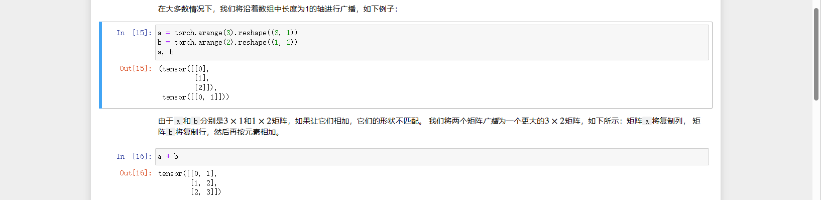
It essentially becomes
1 | tensor([[0], tensor([0,0], |
and then the transformed
1 | tensor([[0, 1]]) |
to perform operations
To perform operations, it must satisfy: for instance, a 3x1 matrix and a 1x2 matrix can perform matrix operations.
Indexing and Slicing
This part is relatively simple and is essentially the same as Python syntax.
1 | X[-1] # Output the last row |
Saving Memory
In Python, the memory address of the result object changes after performing an operation.
When the reuse rate of this object is high and the data volume is large, we need to consider saving memory. This means assigning all values of a new object of the same shape to zero and then putting the result of the operation into this new object. The specific situation is as follows:
1 | Z = torch.zeros_like(Y) |
Converting to Other Python Objects
It’s easy to [convert tensors defined by deep learning frameworks to NumPy tensors (ndarray)] and vice versa. Torch tensors and NumPy arrays will share their underlying memory, so in-place operations will change both tensors.

CN
教材地址:https://zh-v2.d2l.ai/chapter_preliminaries/ndarray.html
数据操作
深度学习处理数据的方式大体有两种,以Pytorch为例
- python的NumPy计算包:只支持cpu计算
- Pytorch的Tensor:支持GPU加速计算
注意,我们要处理的数据,即n维数组,也称为张量(tensor)
入门
我们先进入jupyter环境
1 | jupyter notebook |
然后找到对应章节的ipynb文件,这里是数据操作
接着我们可以在导入torch包后进行调试
当然你也可以修改代码进行调试
这里只提醒一点:为了便于理解,我们可以想象在一个 torch.zeros(...) 中有几个参数即有几维的张量,以上面为例,
从右侧看起,第一个3表示一个大小为3的向量,由一层[]包裹,
接着看到第右侧起二个4,代表四个一维向量构成的二维矩阵,外侧也由一层[]包裹,
第三个2也是如此,代表两个二维矩阵构成的三轴张量,外侧也由一层[]包裹,看是不是很简单。
牢记从右往左看的思想
1 | torch.arange(12) #创建从0开始的12个整数的行向量 |
运算符
对于任意具有相同形状的张量, [常见的标准算术运算符(+、-、\*、/和\**)都可以被升级为按元素运算]。
按元素运算简单理解就是,可以只对一个张量的某一个特定元素进行点对点运算
1 | x = torch.tensor([1.0, 2, 4, 8]) |
广播机制
本质就是扩充
在两个形状不同的张量进行运算的时候,就会触发广播机制,如下面的案例
实质一个就是
1 | tensor([[0], tensor([0,0], |
在和进行了变换的
1 | tensor([[0, 1]]) |
进行运算
要进行运算需要满足:如 3x1 的矩阵和 1x2 的矩阵可以运算,即矩阵运算
索引和切片
这部分相对较简单和python语法基本一致
1 | X[-1] #输出倒数第一行 |
节省内存
python中计算结果对象的内存地址在进行一次运算后会改变
当这个对象的复用率很高且数据量比较大时,我们就要考虑采用节省内存的方式,即将一个新的形状一样的对象全部赋值为零,再将运算的结果放到这个新的对象中,具体情况如下:
1 | Z = torch.zeros_like(Y) |
转换为其他Python对象
将深度学习框架定义的张量[转换为NumPy张量(ndarray)]很容易,反之也同样容易。 torch张量和numpy数组将共享它们的底层内存,就地操作更改一个张量也会同时更改另一个张量。